Understanding and analyzing the runtime characteristics of the garbage collector (GC) is important for several reasons. Firstly, GC pauses can directly impact the responsiveness of your application. By understanding how the garbage collector is performing, you can optimize its settings to reduce these pauses. In general, frequent long GC cycles may indicate that the heap is too small, or that too many temporary objects are being created.

With the help of the garbage collector probe you can solve these problems and make more informed decisions when tuning your JVM settings, such as selecting the appropriate garbage collector, heap size, or other JVM parameters.

The garbage collector probe has different views than the other probes and also uses a different data source. It does not obtain its data from the profiling interface of the JVM but uses JFR streaming to analyze GC-related events from the JDK flight recorder. Because of the dependency on JFR event streaming, the GC probe is only available when you profile Java 17 or higher on a Hotspot JVM. When you open JFR snapshots, the exact same probe is available, regardless of the used Java version.

Garbage collections view

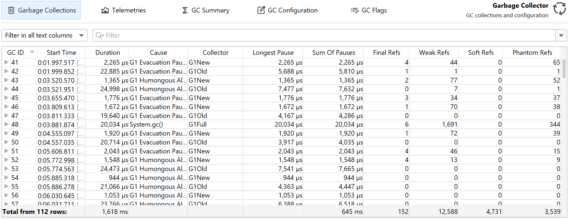
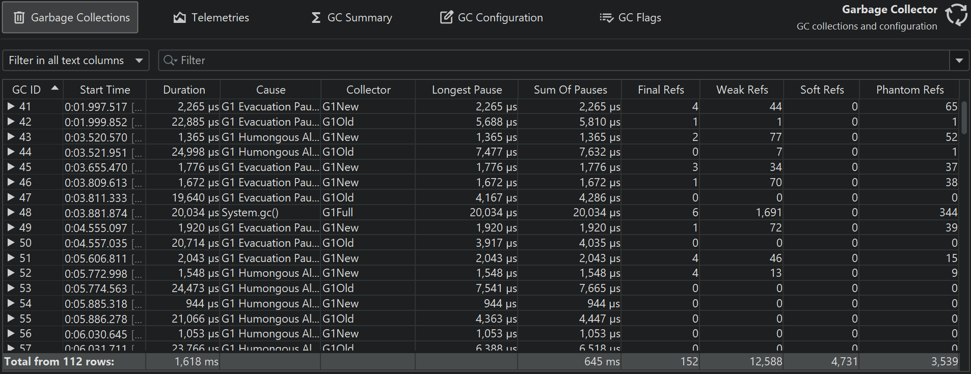
The main view in the garbage collector probe is the "Garbage collections" table. It shows all recorded garbage collections as rows with their most important metrics as columns.

The "Cause" column shows you why a garbage collection was triggered. For example, a call to System.gc() triggered a full garbage collection. You can see that from the associated "G1Full" value in the "Collector" column. It also caused a substantial pause of 20 ms which is why it is generally not a good idea to call System.gc(). Other causes trigger the collection of the young generation space ("G1New") or the old GC collection of the G1 collector ("G1Old") that cleans up unreferenced objects in the old generation. You can see that the old GC collections consistently take longer than the young generation collections although the young generation collections collect more objects.

Collected references with special GC handling are shown as "final", "weak", "soft" and "phantom" references in separate columns.

The reason there are separate columns for the longest pause and the sum of pauses is that each garbage collection is composed of multiple phases that produce separate pauses. Also, the "Duration" of a garbage collection is not equal to the sum of pauses, because a garbage collection only partially pauses the JVM while it is executing. You can see that the "G1Old" collections in the screenshot only pause for about a fifth of their duration.

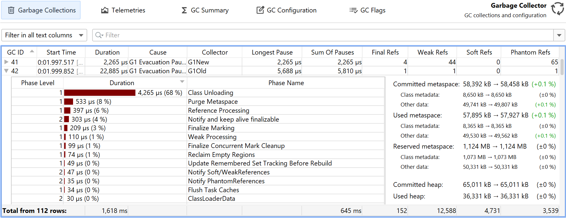
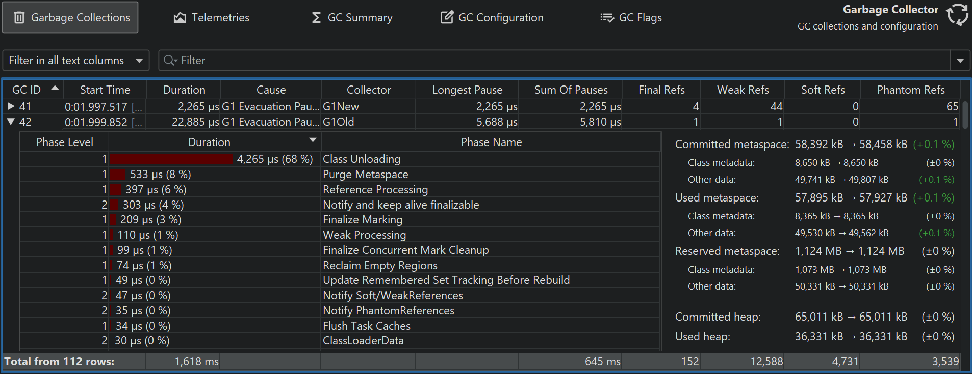
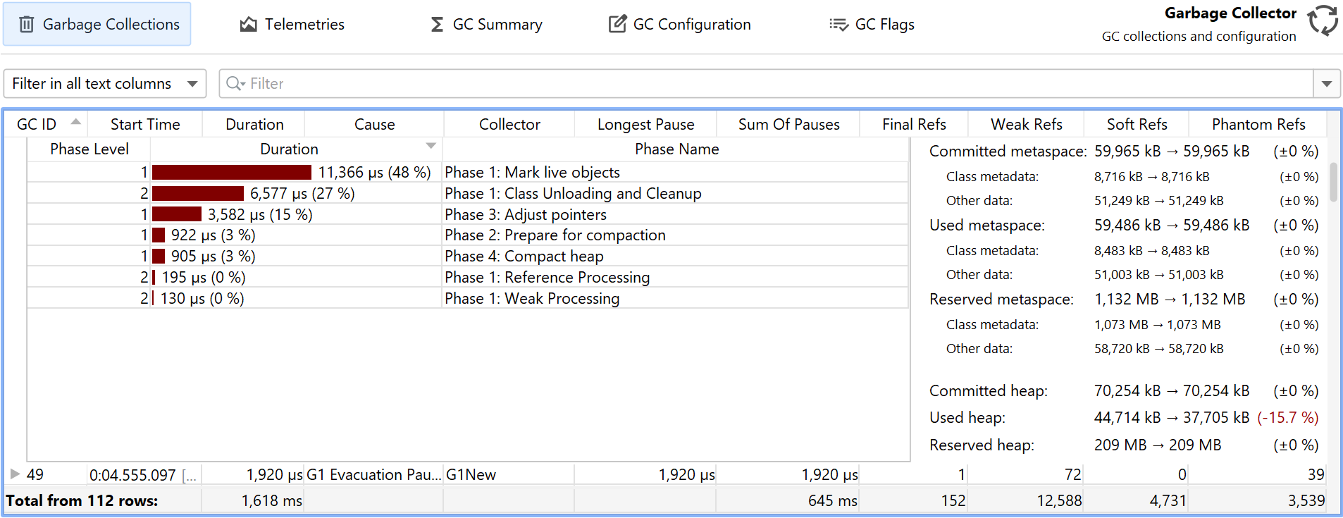
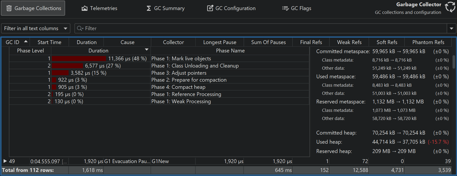
To inspect the various phases of a garbage collection, you can toggle the tree icon in the "GC ID" column.

In the screenshot above, a mixed GC collection of the G1 collector ("G1Old") was expanded. You can see that most of the time is spent in "Class Unloading", which does not pause the JVM. On the right, you can see further statistics for the garbage collection. Here, the used heap stayed the same while the used metaspace went up by 0.1%.

The phases of each collector are different. In the screenshot above, a full collection is shown. It spends a lot of time marking live objects in the entire heap. At the end of the collection, the used heap was reduced by 15.7%, while the metaspace remained the same.

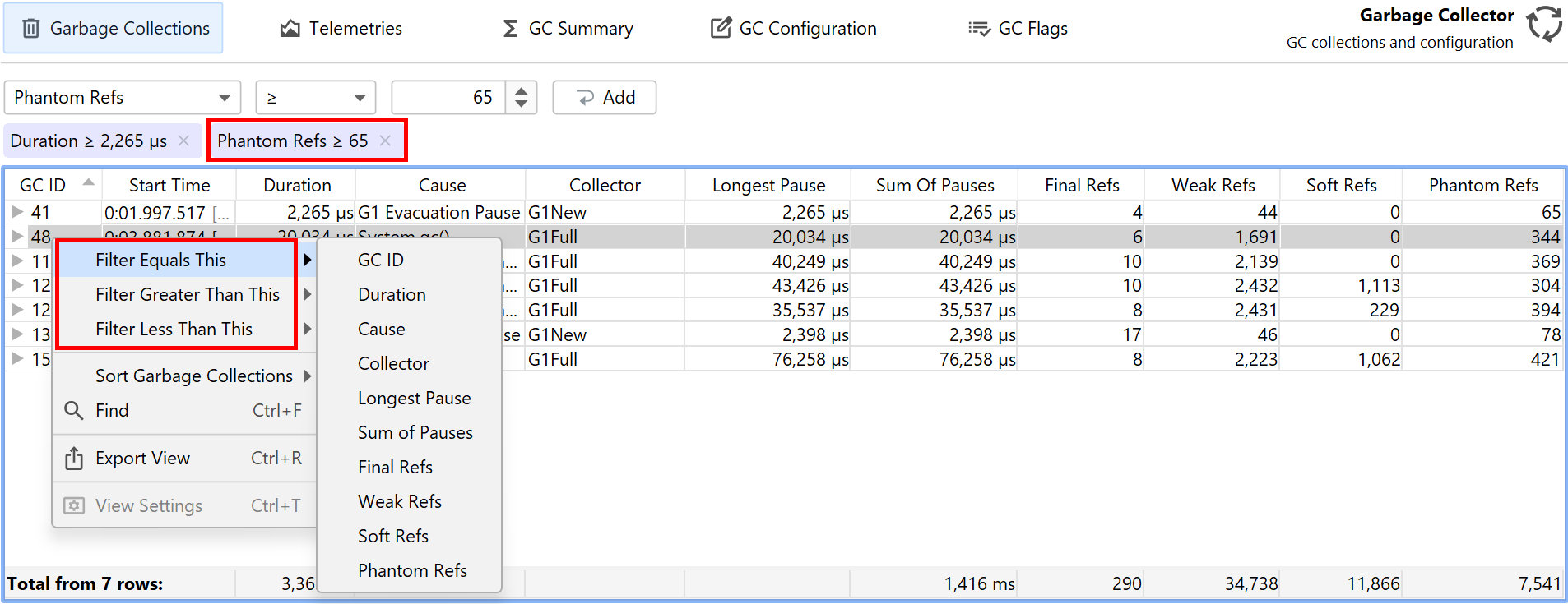
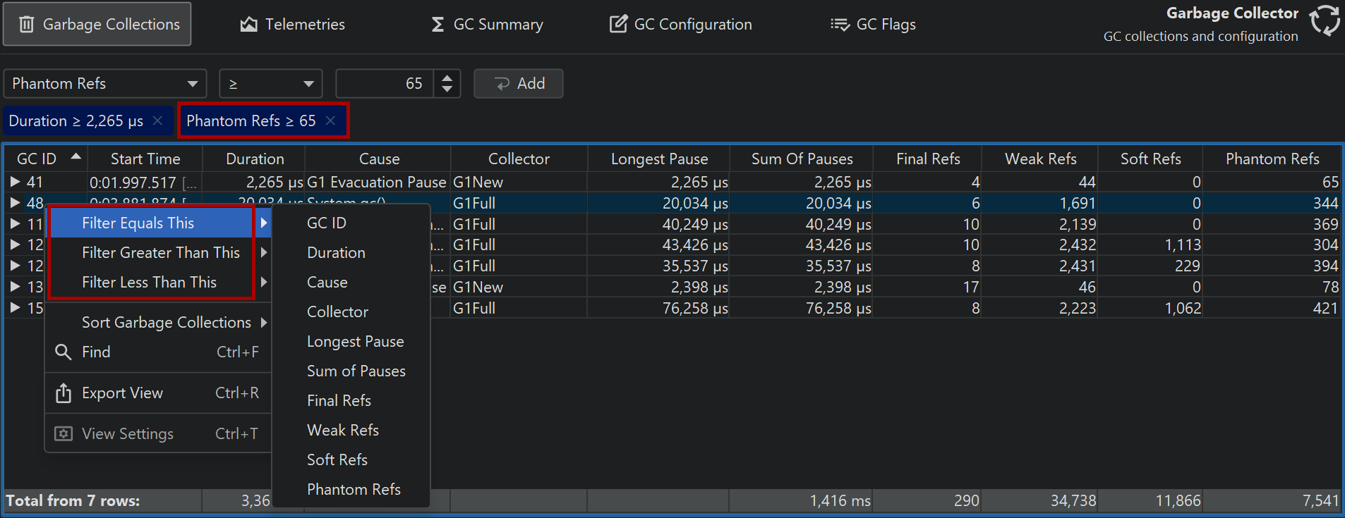
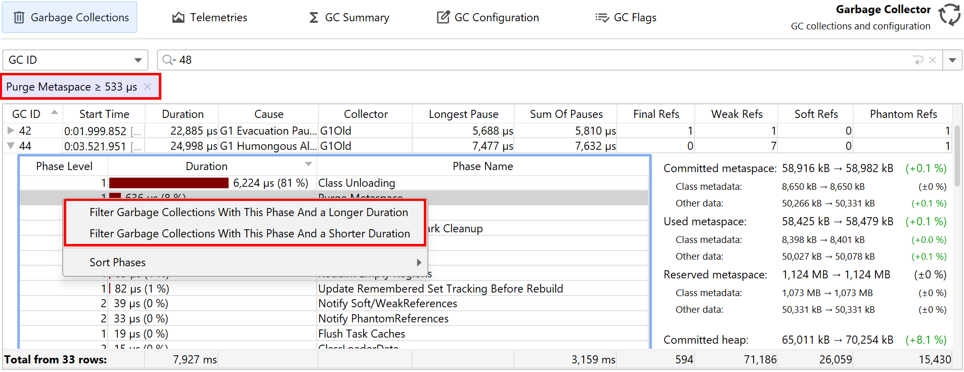
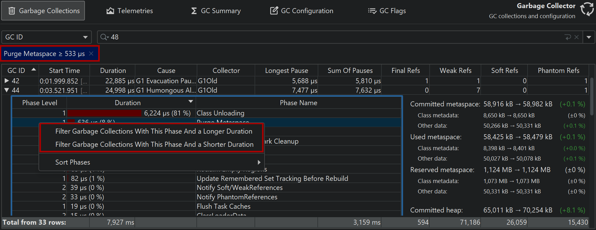
While analyzing garbage collections, filtering is an important tool to compare different subsets of garbage collections. At the top of the table, there is a filter selector that lets you choose any column and configure a corresponding filter. An easier way to see similar garbage collections is to use the context menu on the table and select a filter condition based on the column values in the selected row.

You can add multiple filters to narrow down the garbage collections of interests. Active filters are shown as labels at the top of the table. It is also possible to add filters from the nested GC phases tables.

Telemetries

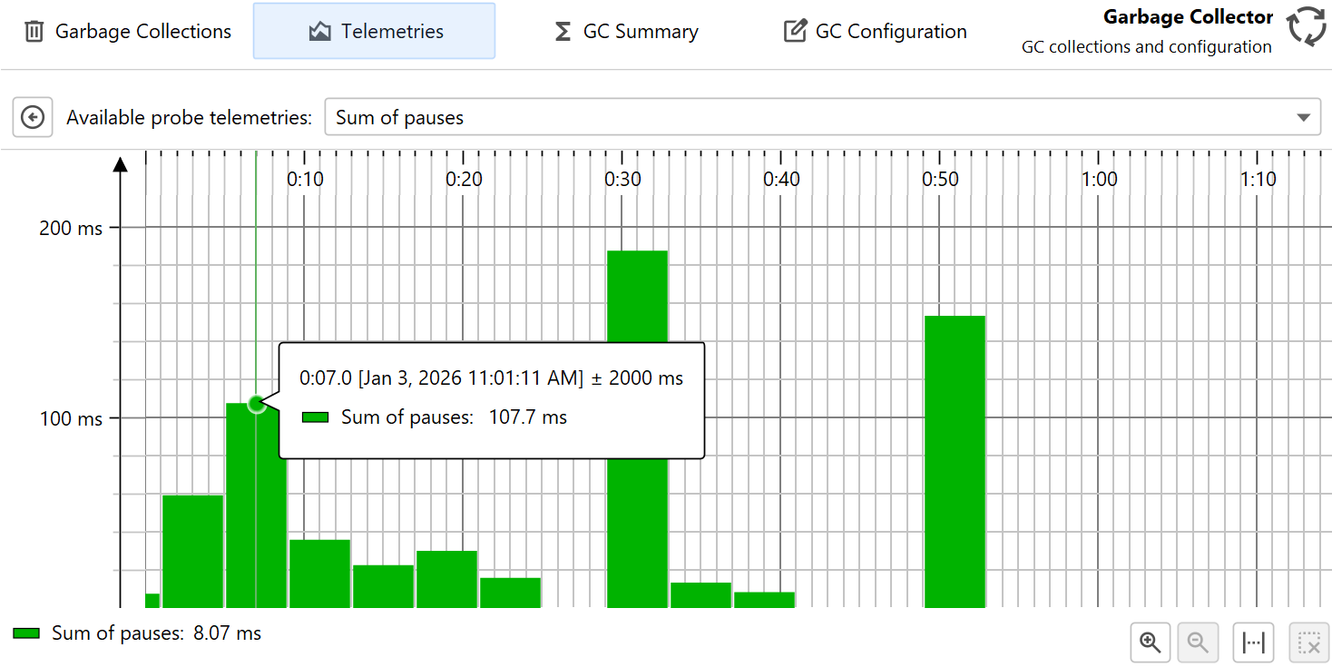
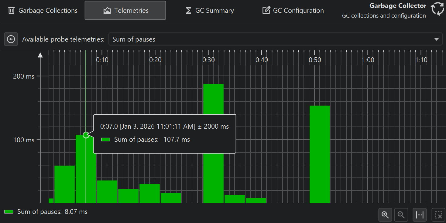
The GC probe produces a number of telemetries which are available in the "Telemetries" probe view.

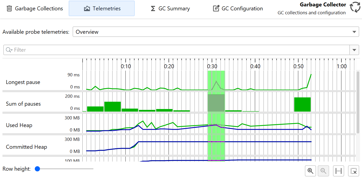
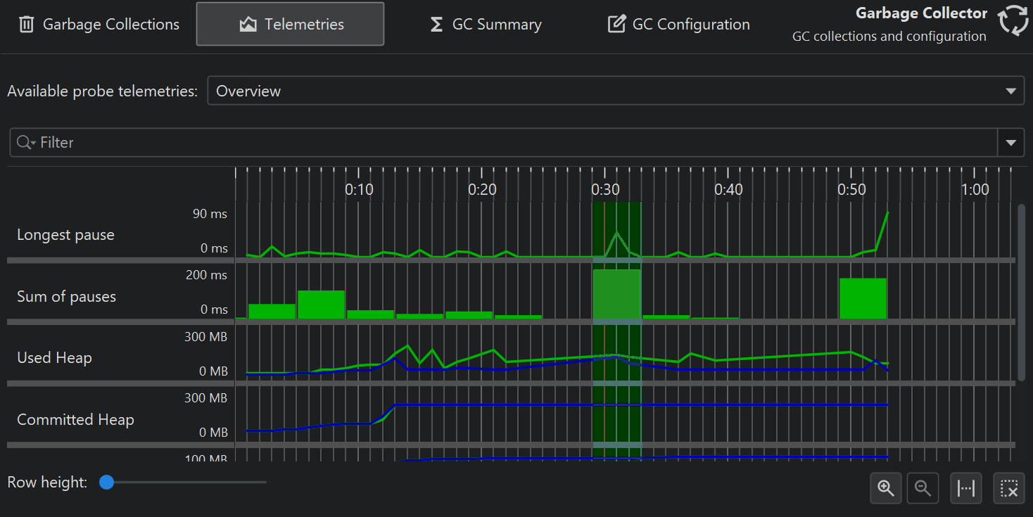
If you are interested in minimizing GC pauses, the "Longest pause" telemetry at the top will be the most interesting one. You can drag along the time axis of the telemetry to select the corresponding garbage collections in the "Garbage Collections" view. For better vertical resolution, you can select a single telemetry from the drop-down at the top or by clicking on the name of the telemetry.

In the screenshot above you can see the sum of pauses over time. JProfiler presents summable measurements by building a histogram of the recorded data. The bin width depends on the available horizontal space, so histogram bins will change depending on the zoom level and, if "scale to fit" is enabled, depending on the width of the window. What stays the same is the total area under all histogram bins.

The heap and metaspace telemetries are based on the statistics that you can see when expanding a garbage collection. This means that the data is not regularly sampled like for the memory telemetries in a full profiling session. If no garbage collection occurs during a time period, there will be no data. For a JVM with little allocation activity, there can be long stretches along the time axis where the graph is just interpolated between two garbage collections.

Each of these telemetries has two data lines: "Before GC" and "After GC". The differences are typically large for the "Used Heap" telemetry. At each time, you can see how much work the garbage collection has performed by comparing the values of the two data lines. You can look at the tooltip to get the precise values. For the "Committed heap" telemetry and the metaspace telemetries, the differences between both lines will often be small.

If you are analyzing a JFR snapshot, the same data from the jdk.GCHeapSummary JFR event type is also used in the "Memory" telemetry in the telemetry section. In that case, however, both the "Before GC" and "After GC" values are shown in the same data line and data is not aggregated to a once per-second granularity as in the GC probe telemetries, so the graph will look different.

GC Summary

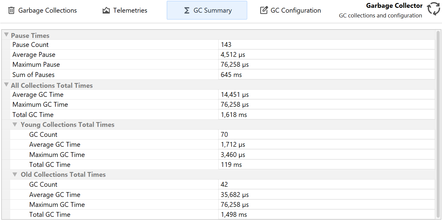
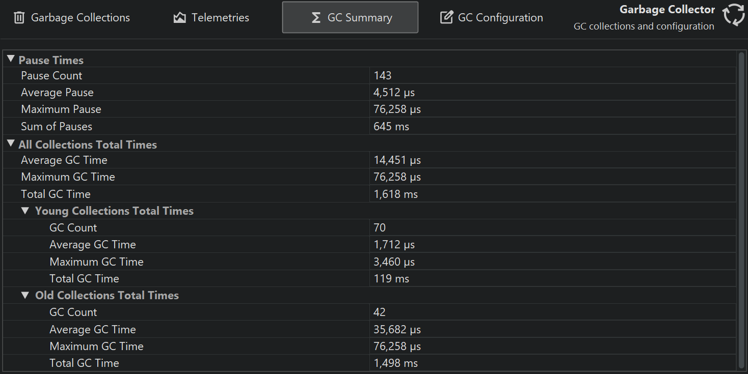
The GC summary shows you measurements that are aggregated over the entire recording period. Each measurement provides the number of garbage collections, as well as the average, maximum and the total values. The most important data at the top are the "Pause times" that directly affect the liveness of your application.

The other top-level category shows the total times of all collections which is then split into two subcategories for young and old collections.

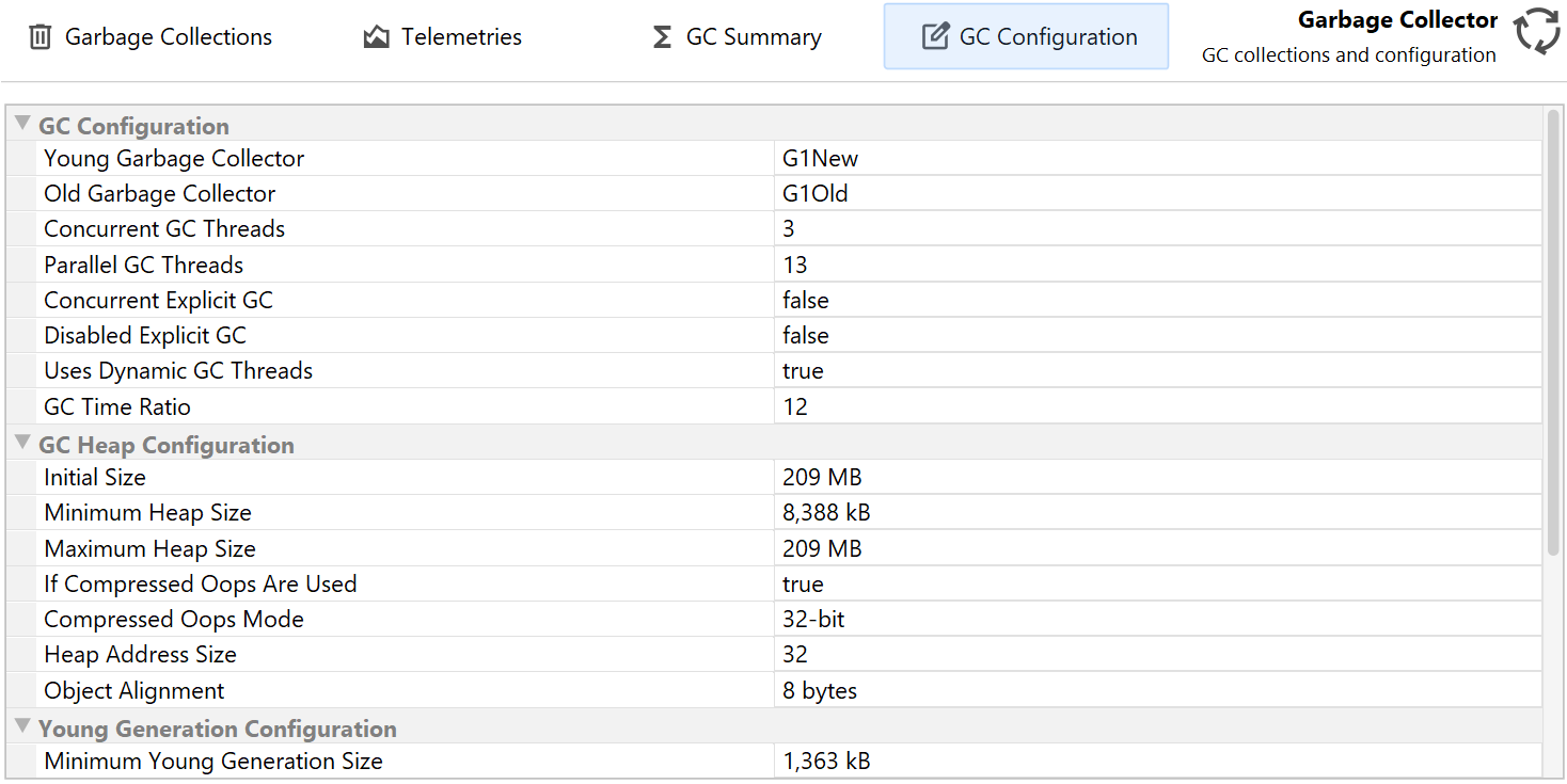
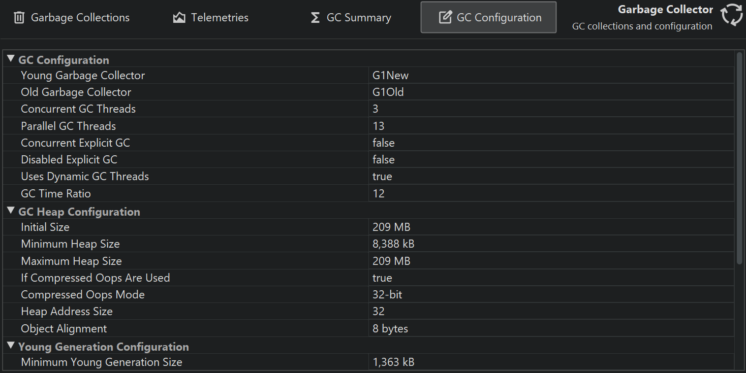
GC Configuration

When you tune your garbage collector, you may want to inspect the common properties that can either be set explicitly or that are set implicitly by the garbage collector itself.

These properties are common to all garbage collectors and help you understand the differences between garbage collectors.

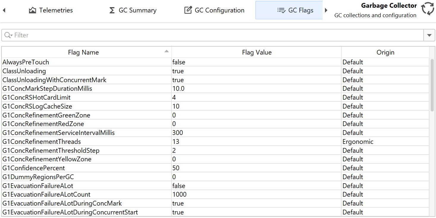
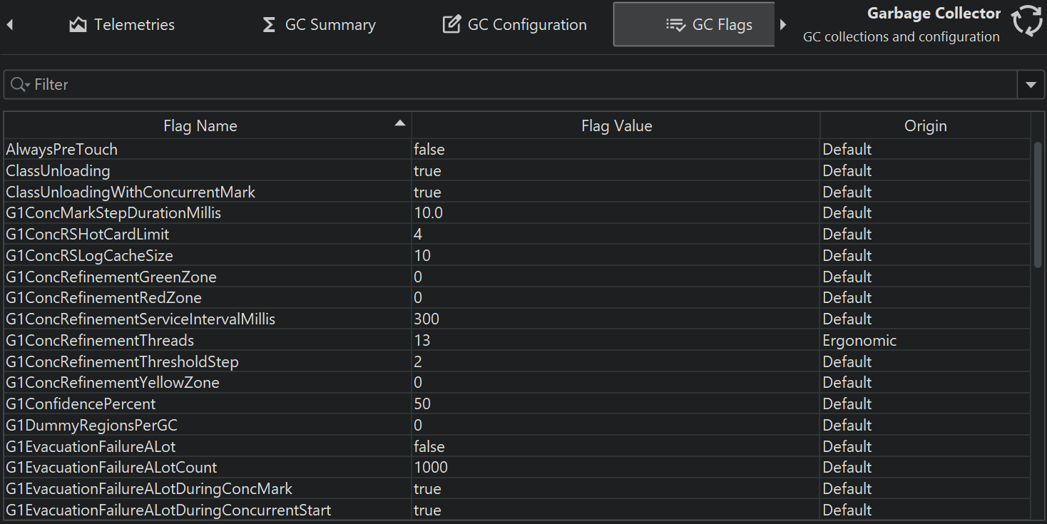
GC Flags

Finally, the GC-specific flags give you an idea what properties of a garbage collector can be tuned and lets you check their actual values.

The "Origin" column shows you how the flag was set. "Default" values have not been modified from the standard settings while "Ergonomic" flags have been adjusted automatically by the garbage collector. If you set specific GC flags on the command line, they will be reported as "Command line" in origin.