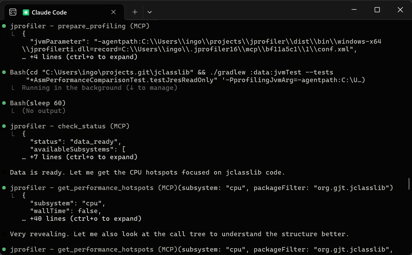
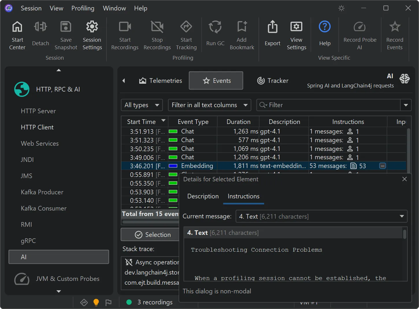
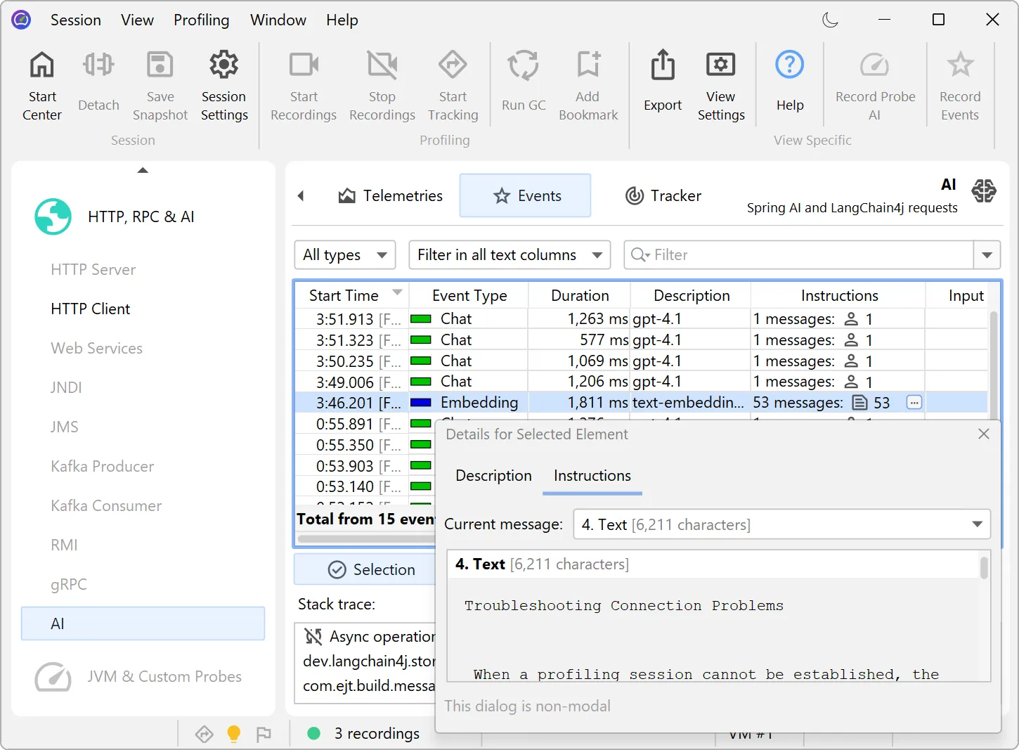
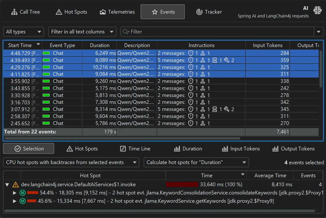
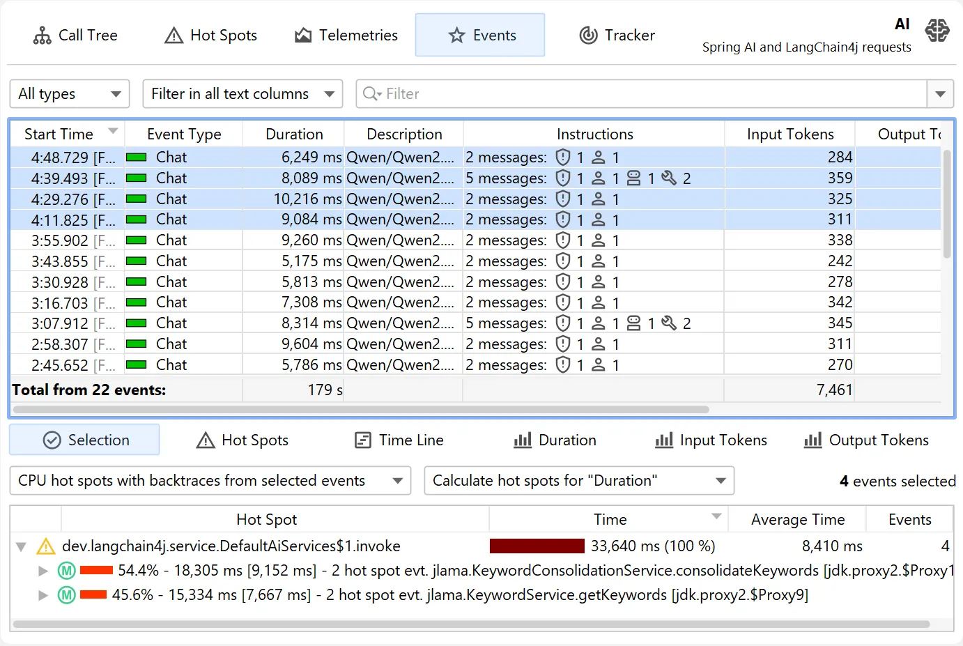
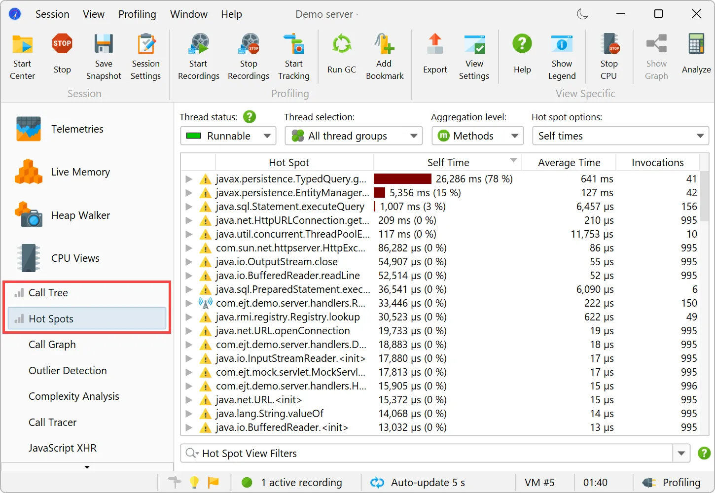
JProfiler 16 introduces an AI probe. The probe measures interactions with LLMs via LangChain4j
and Spring AI.
Chat requests and embeddings are supported and shown in the events view as different event types.
Details for the processed instructions are available in the node detail dialog that can be shown with the hover button in the instructions
column. The instructions column shows statistics for the different instruction types, such as user messages, assistant messages, or
tool messages.
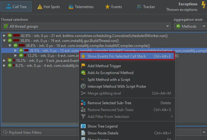
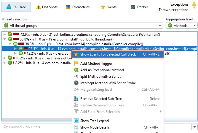
The AI probe is event-centric. You can work with subsets of recorded events in two ways: First, when you select multiple events, the
selection panel at the bottom provides CPU hot spots, probe hot spots, and a probe call tree for the current selection.
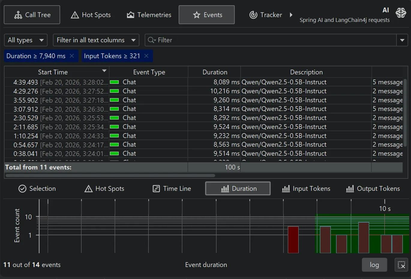
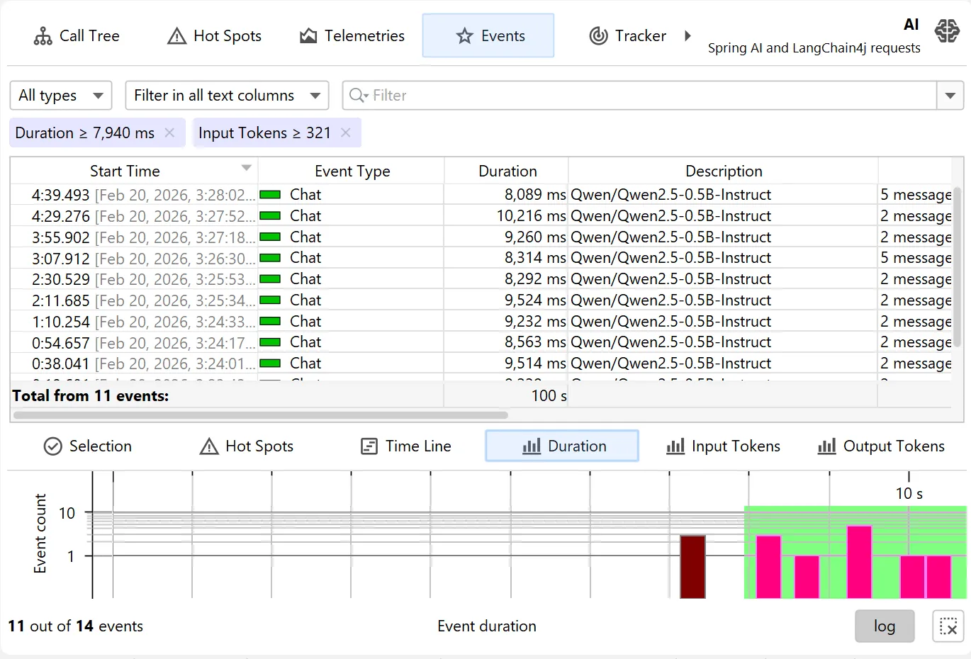
For more thorough investigations, the filter selector at the top and the various tabs in the lower section allow you to restrict the set of events
in the main table and associated views.
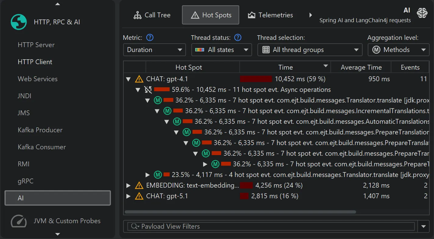
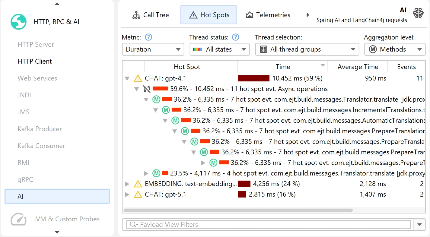
By default, the AI probe identifies hot spots based on the specific model names that processed the request. This data is available
not only in the events view, but also in the hot spot view of the AI probe, even if no events are recorded.
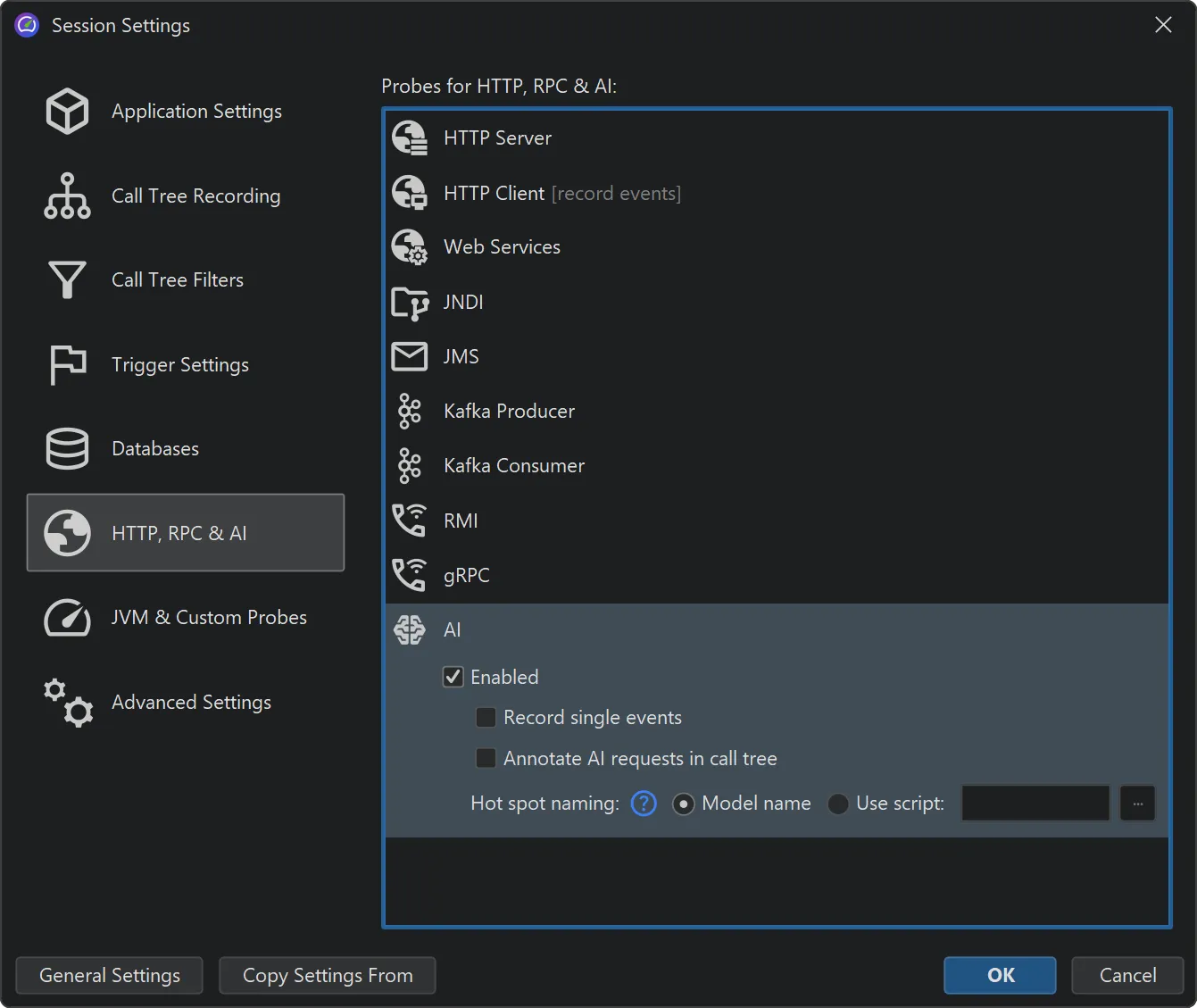
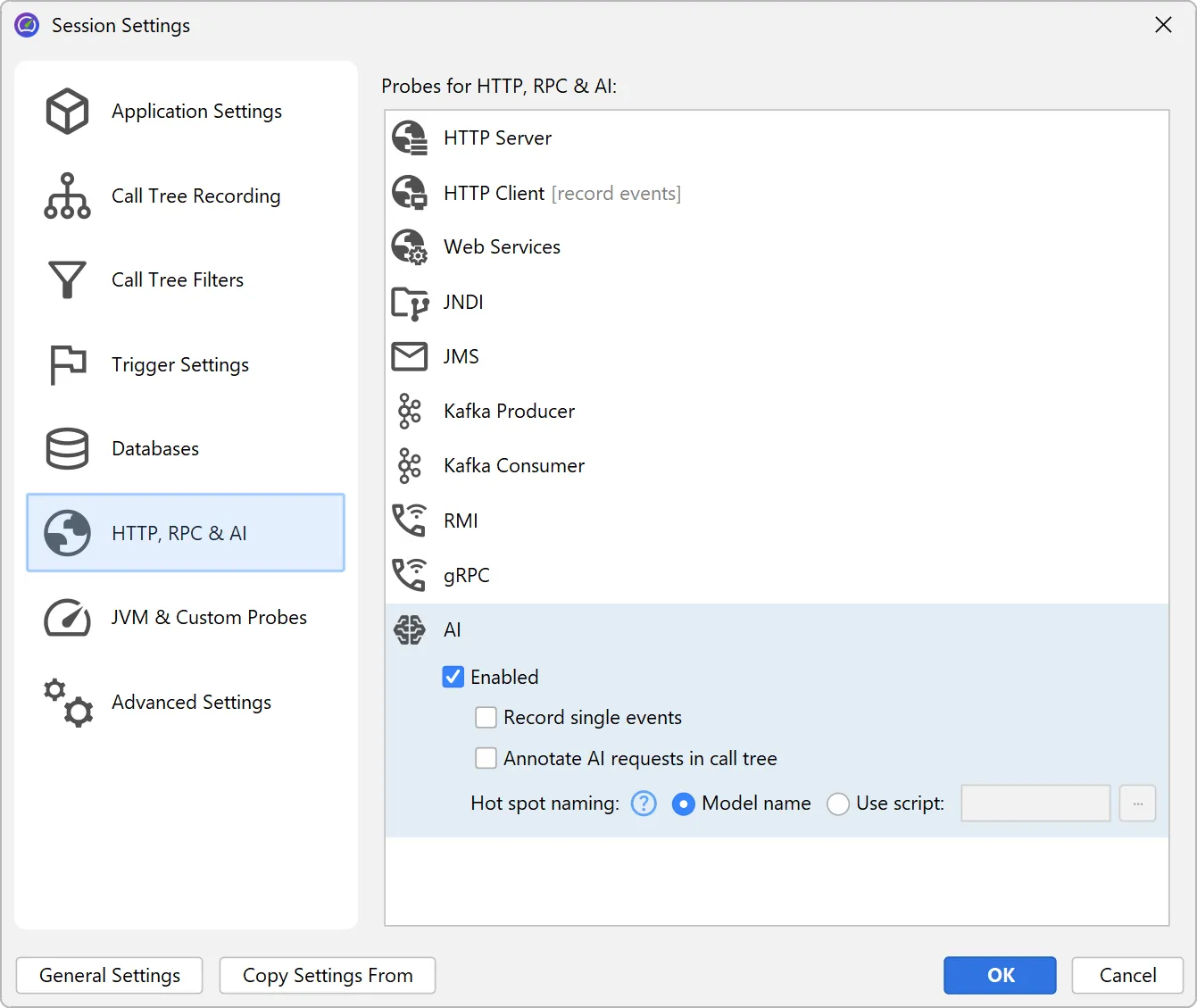
Model name hot spots are only one of many potentially interesting types of hot spots. In the probe settings, you can configure
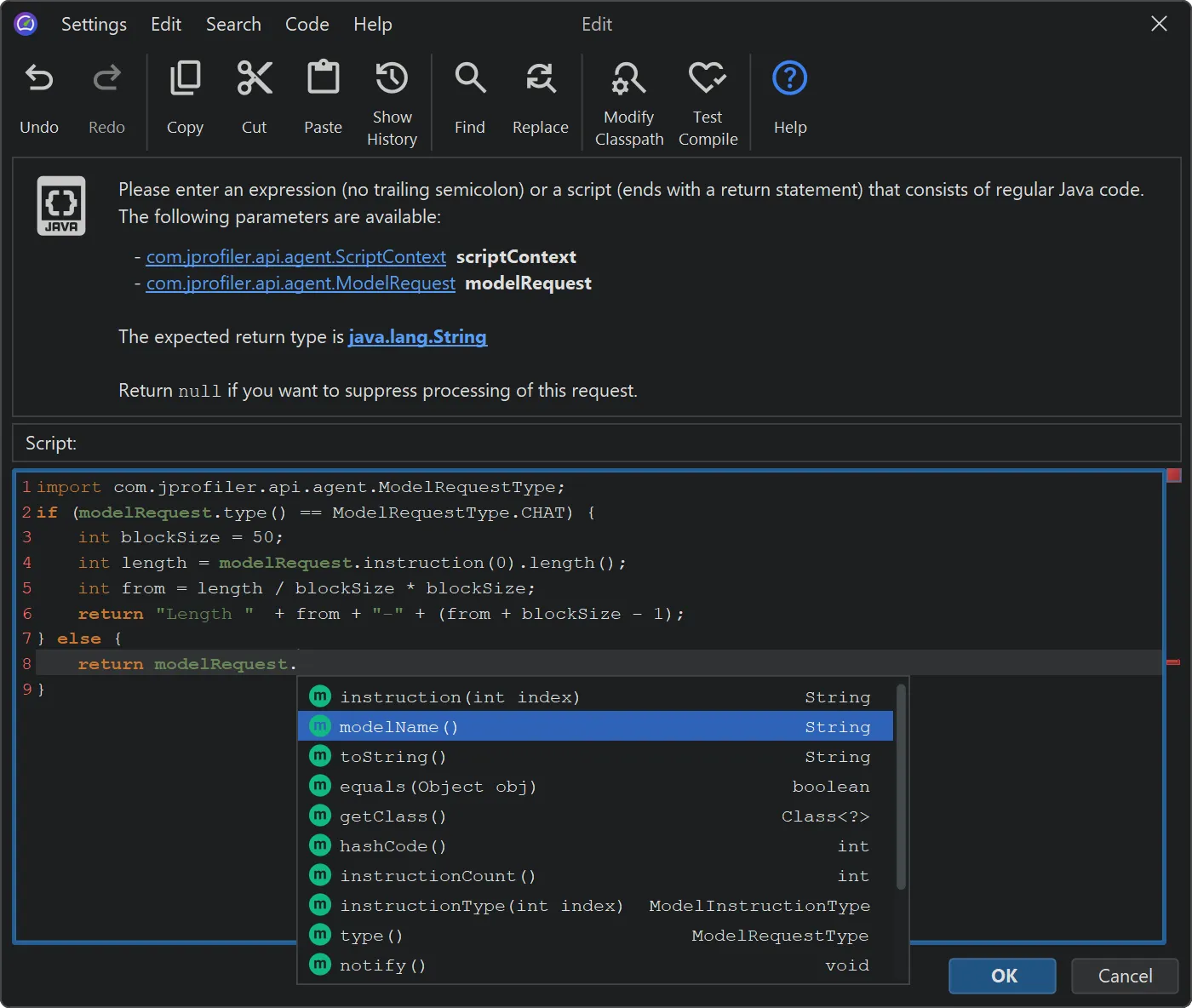
a script to calculate user-defined types of hot spots by entering some Java code in JProfiler's powerful script editor.
When an AI probe event is recorded, JProfiler invokes this script with a ModelRequest parameter. This parameter provides
access to the request type, the model name, and all instructions along with their instruction types.
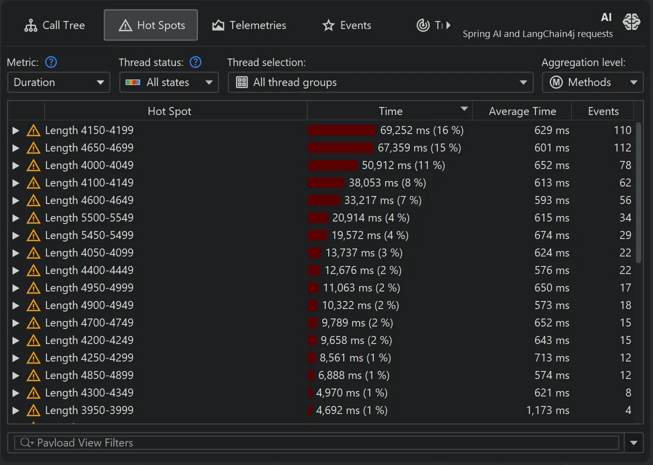
For example, you could define hot spots by grouping prompt lengths into 50-character buckets. The example below demonstrates how this is done.
Since JProfiler displays data live during recording, you can change these settings while profiling and observe the effects immediately.
With the above script, the new hot spots look like this:
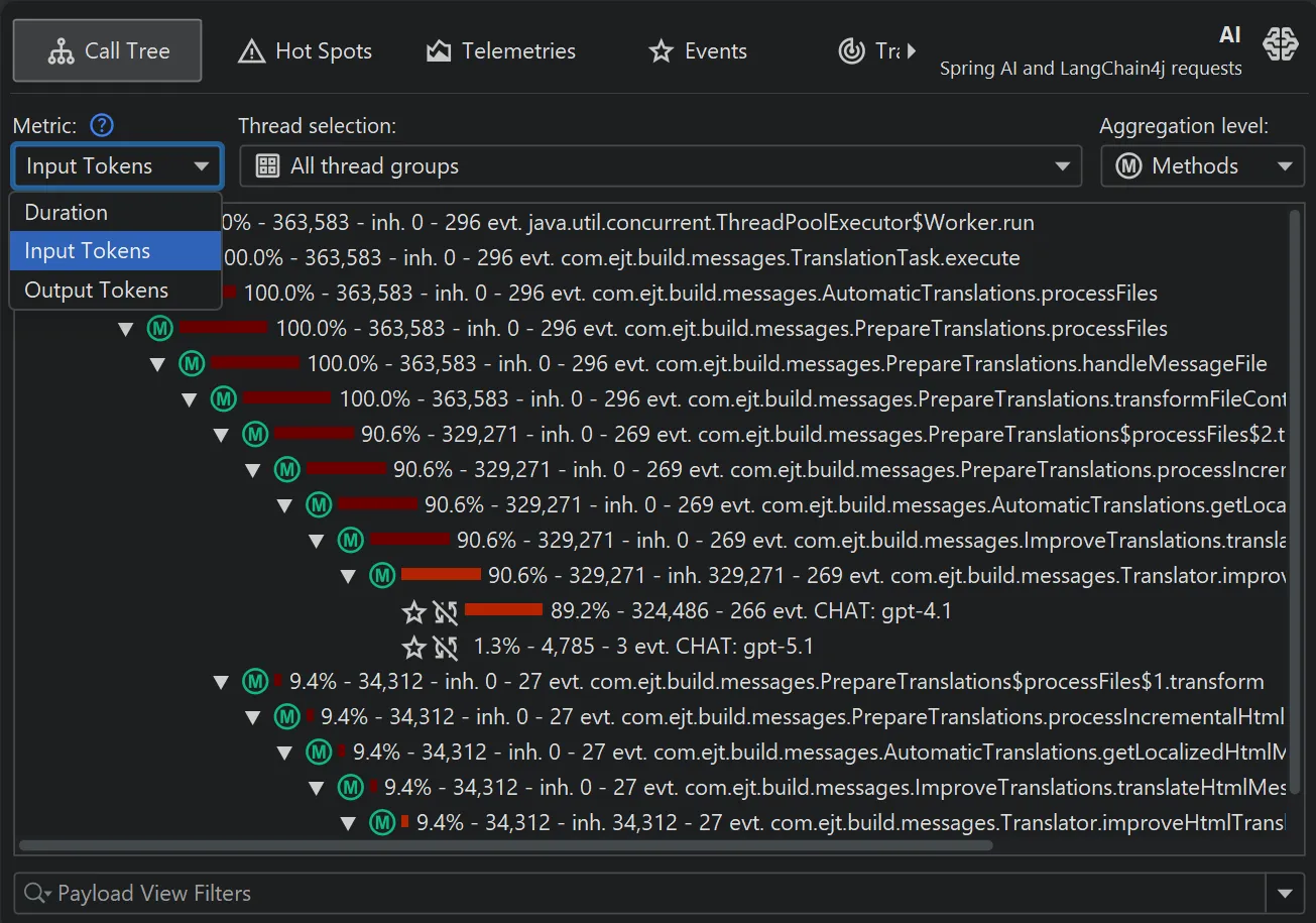
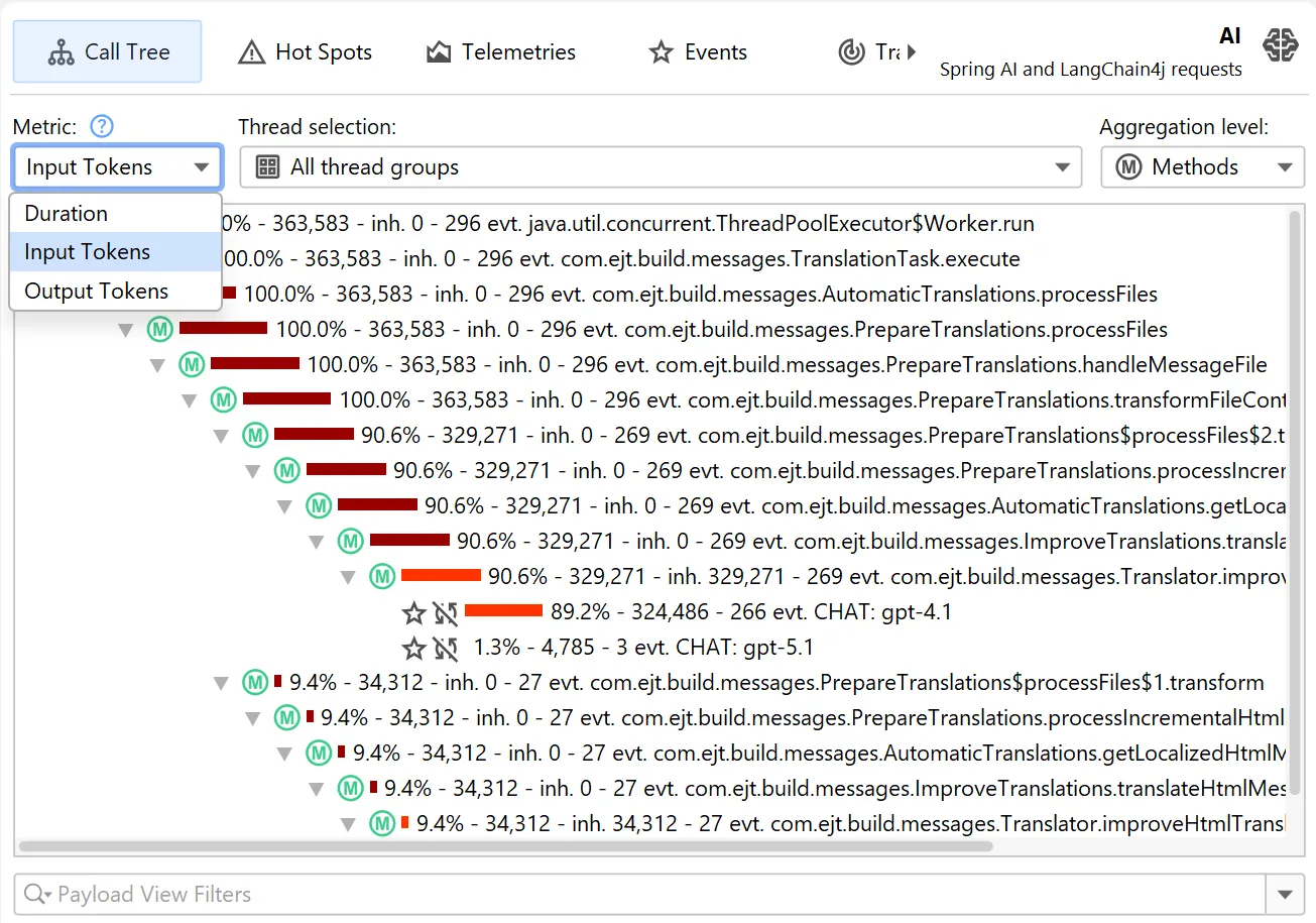
By default, hot spots focus on the request duration, but you can switch the primary measurement to input tokens and output tokens
as well.
This is possible both in the probe hot spots view and the probe call tree view. The probe call tree view shows a top-down view
connecting method calls to probe payloads.
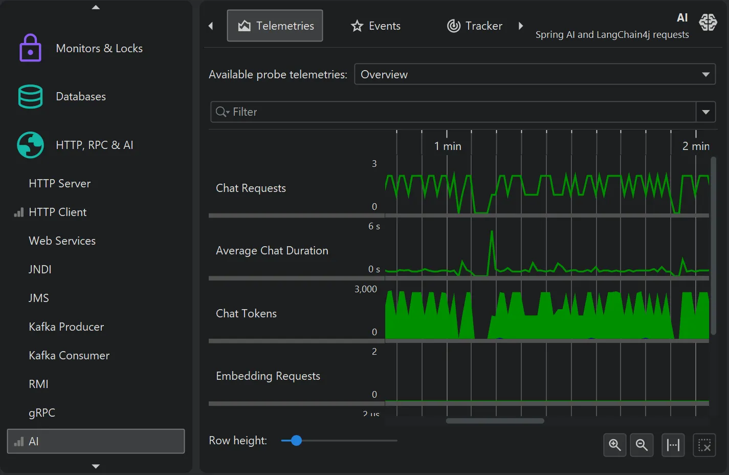
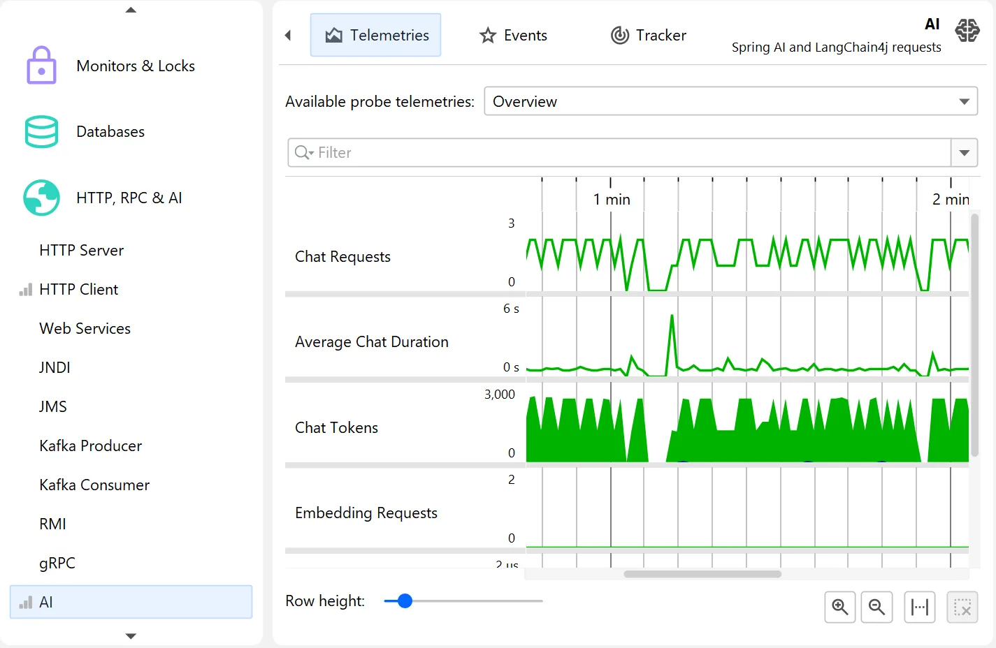
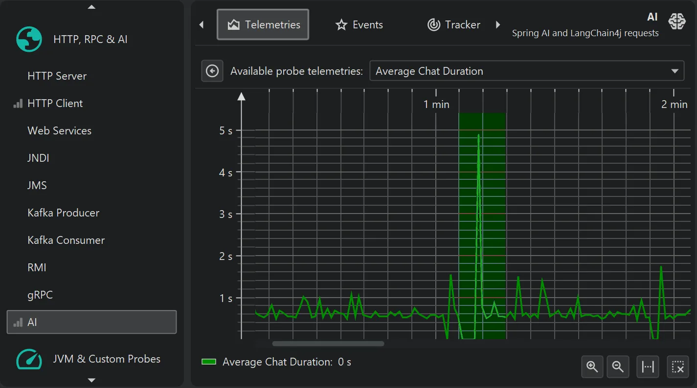
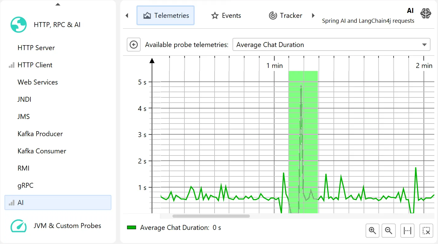
The probe telemetries for the AI probe show request counts, average request duration, and a combined input/output token graph separately for
chat requests and embedding requests.
Each telemetry can be shown separately and can be used to select events for particular areas of interest.
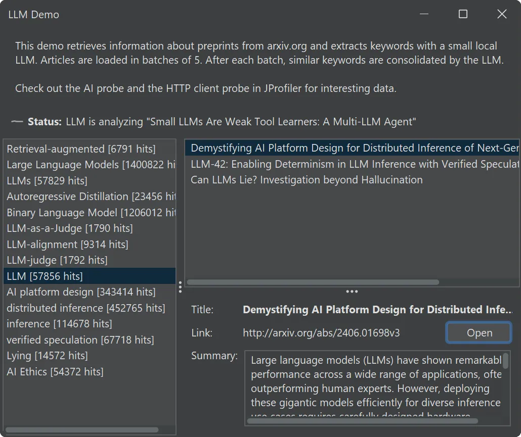
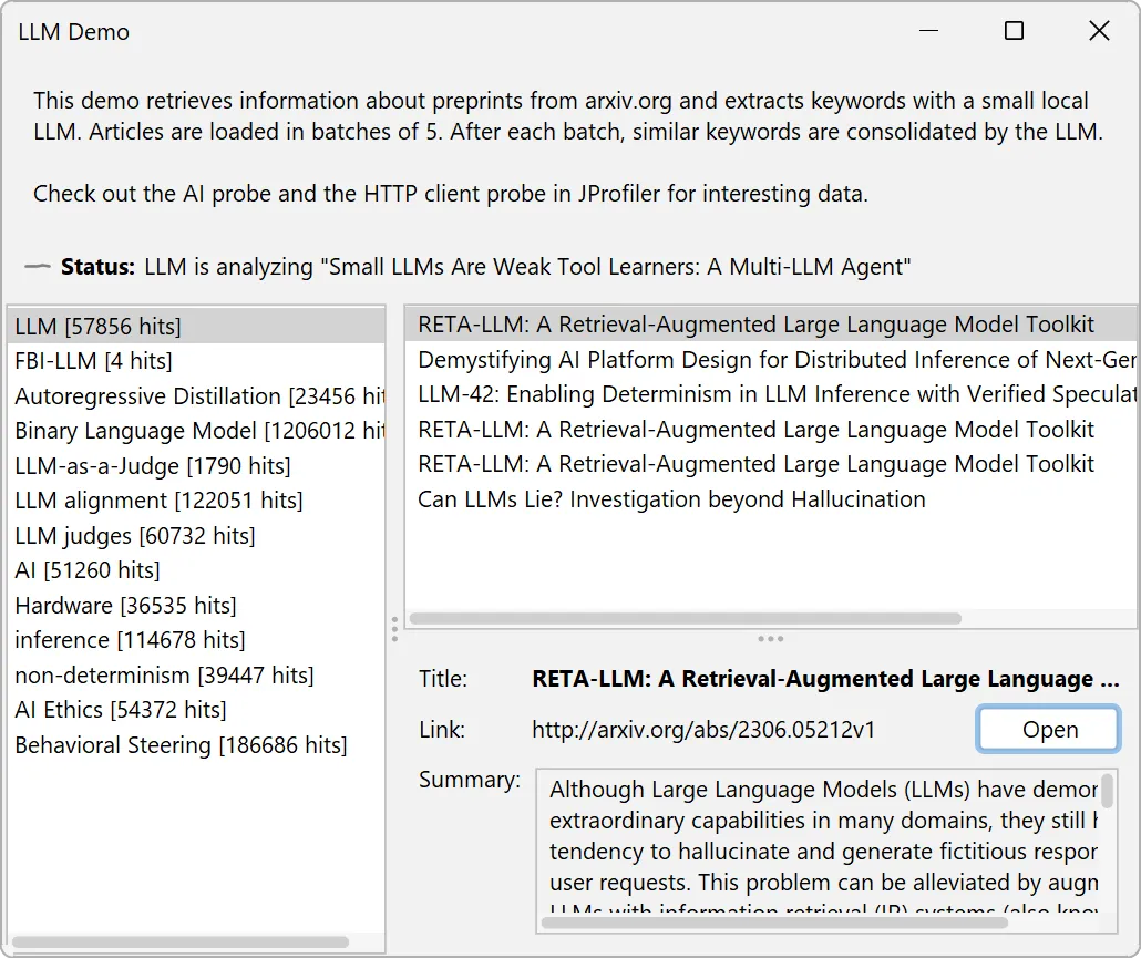
To help you explore the AI probe, JProfiler now comes with an "LLM demo" session.
It uses Jlama, a cross-platform inference engine for Java 21+ and downloads
a 0.5-billion-parameter model from Hugging Face to categorize LLM-related preprints from
arXiv.
The demo features a UI where keywords produced by the LLM are continually inserted and you can explore the associated research papers
on the right.
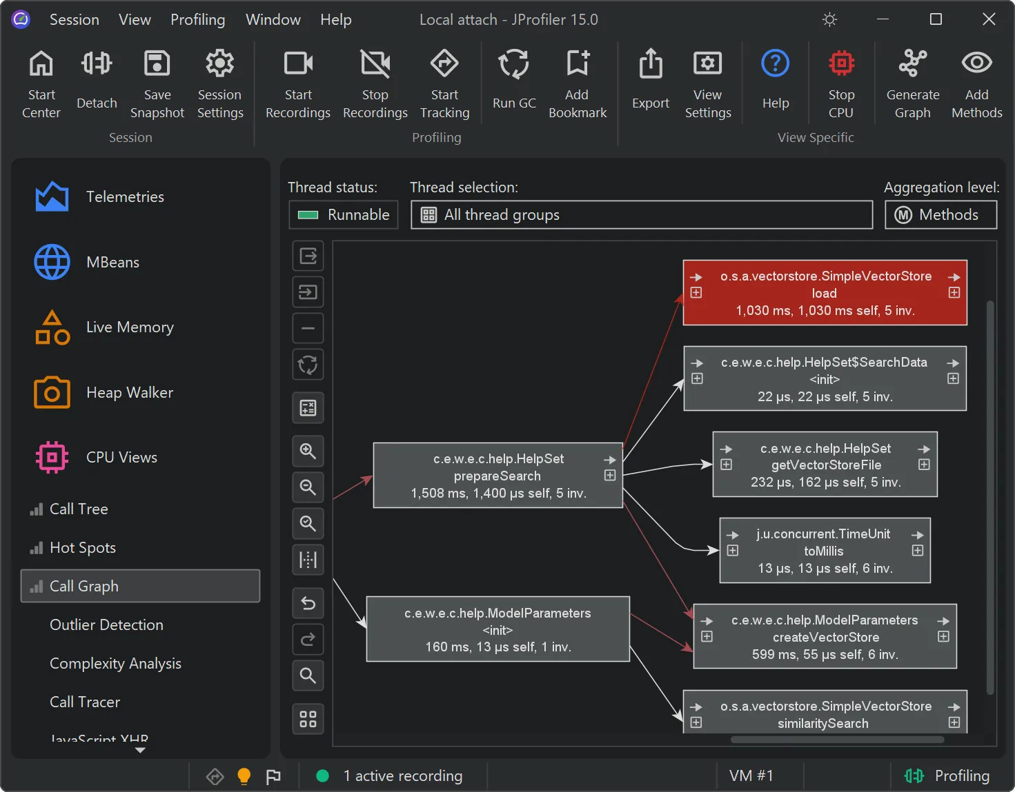
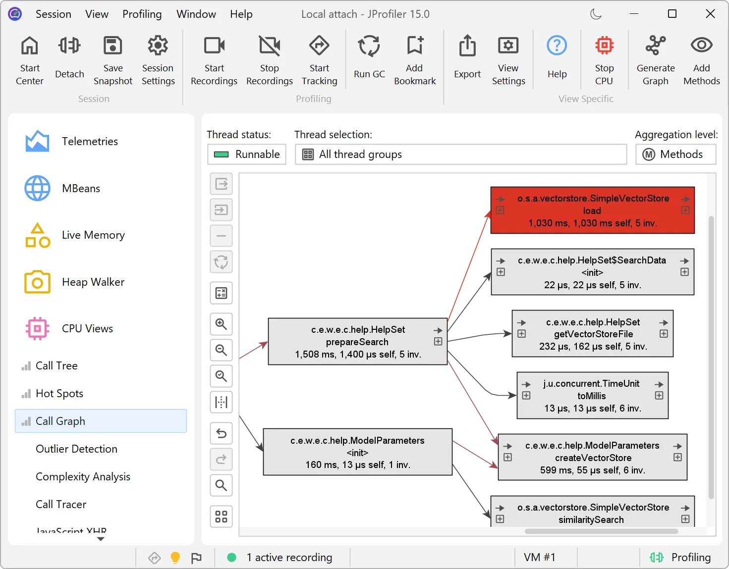
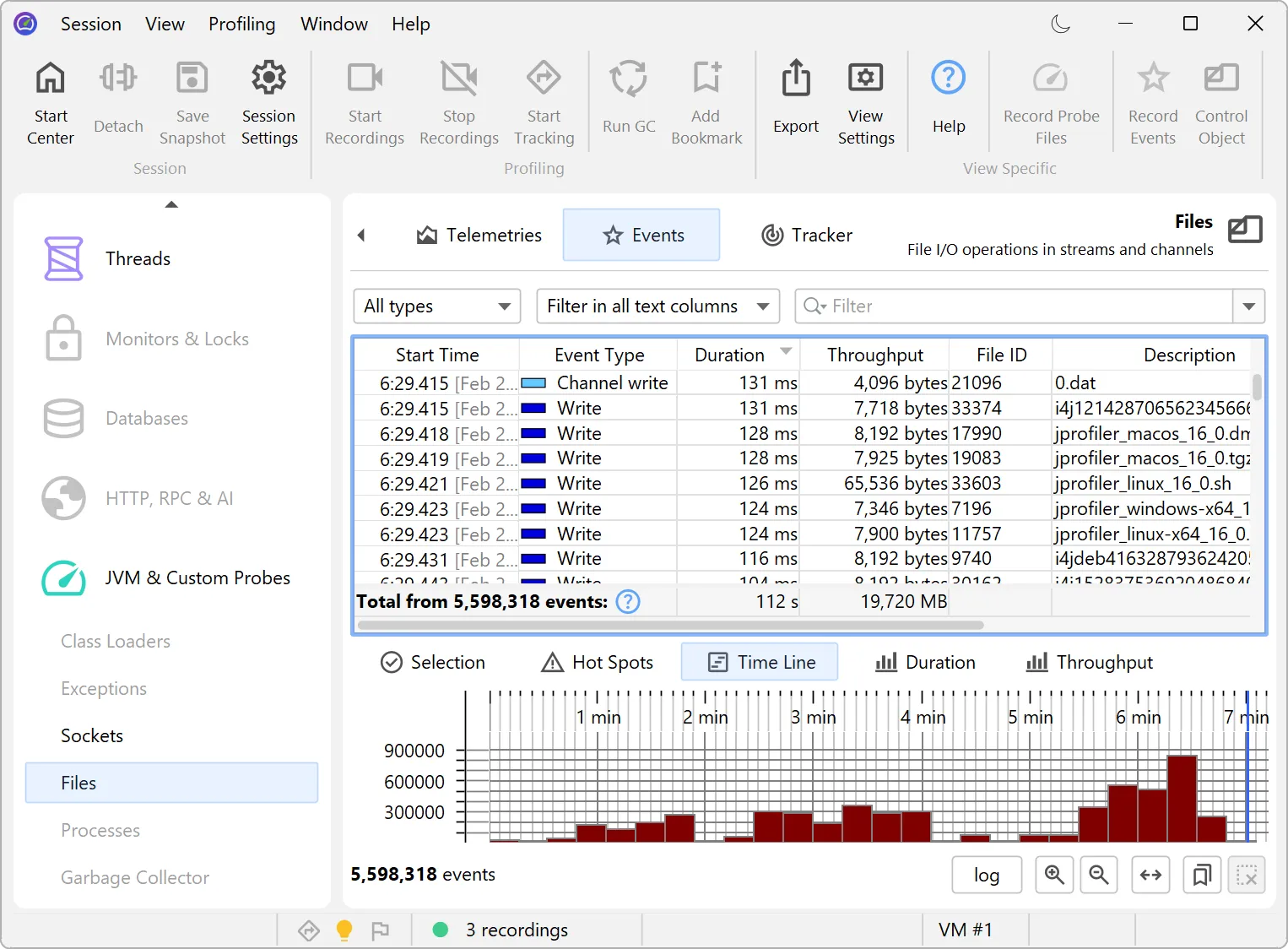
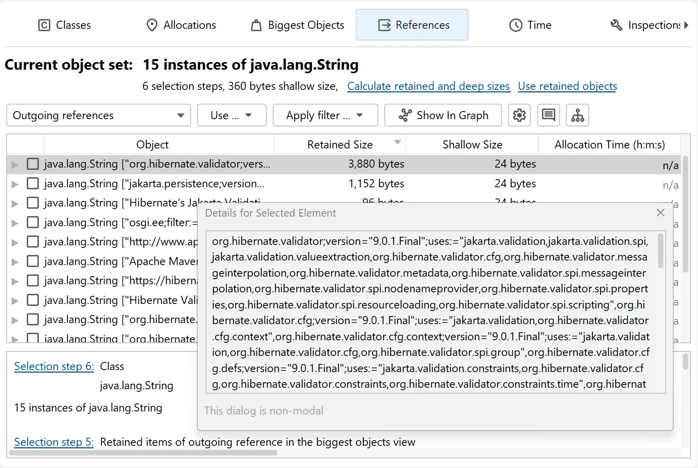
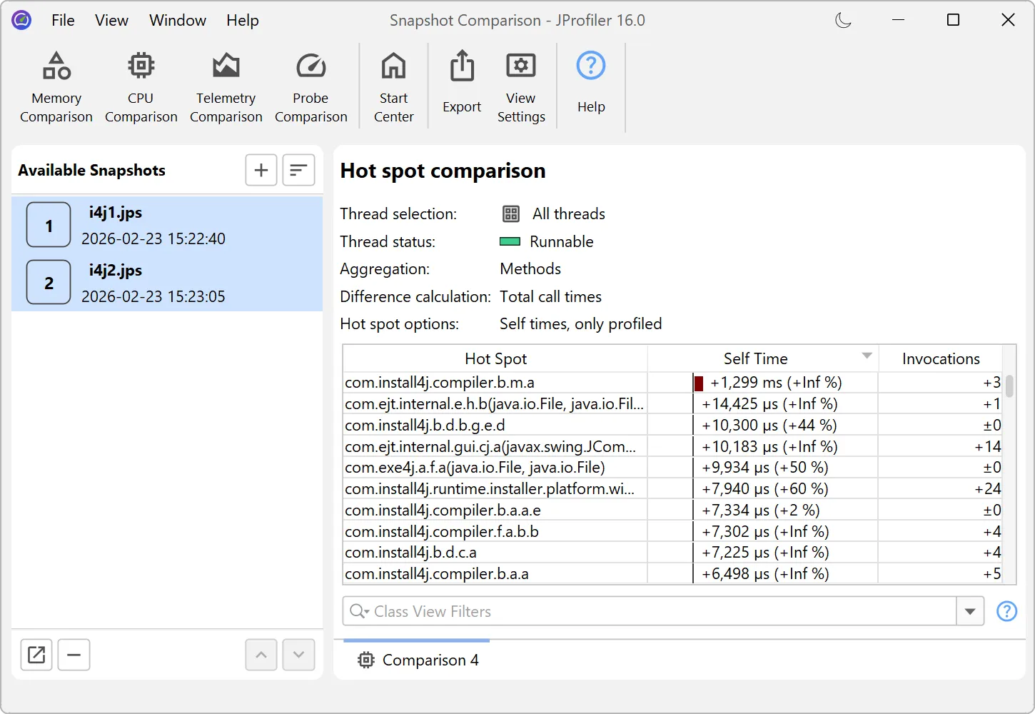
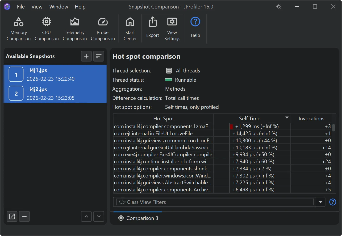
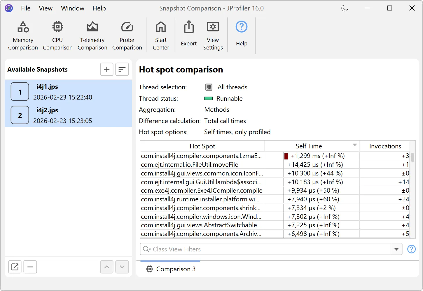
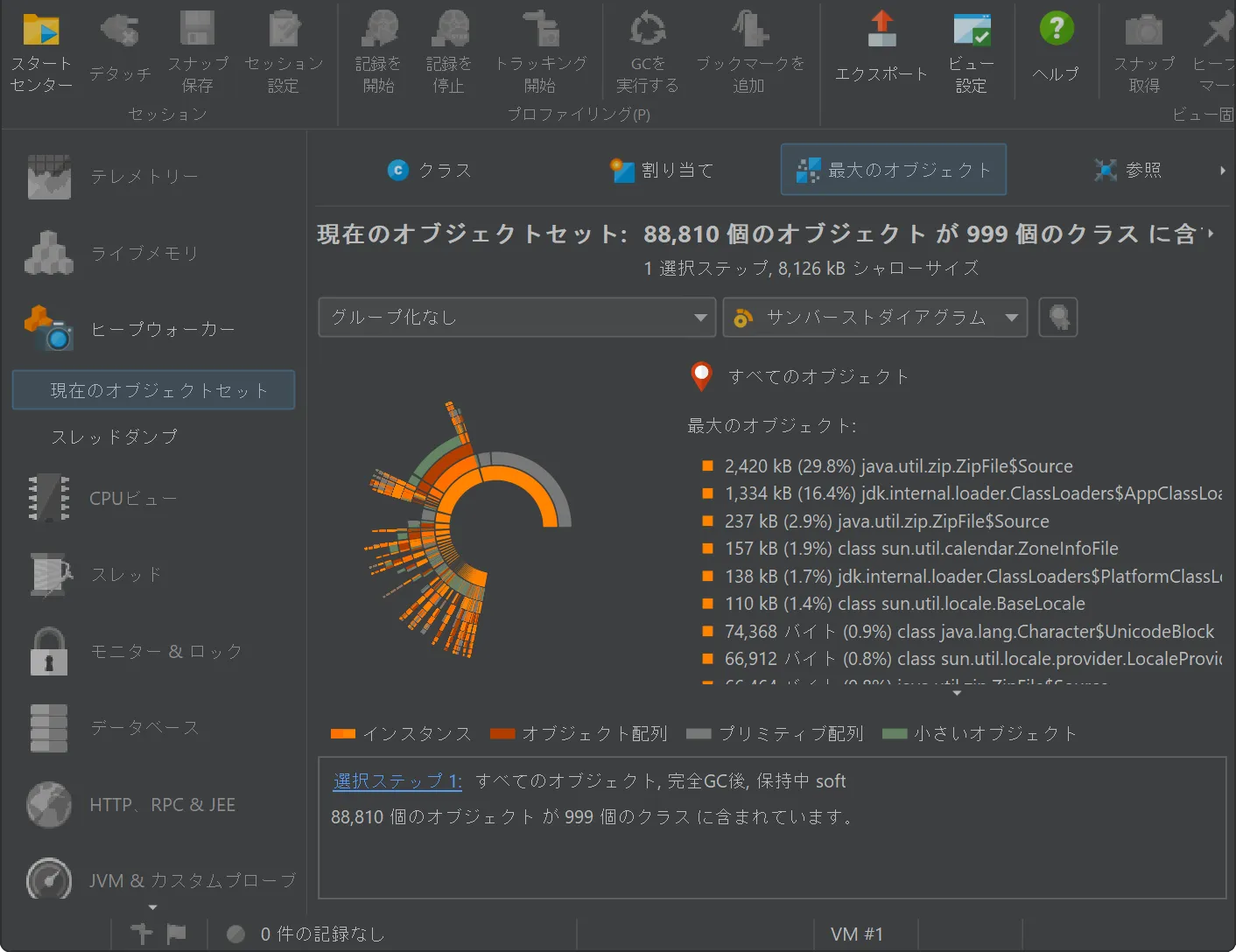
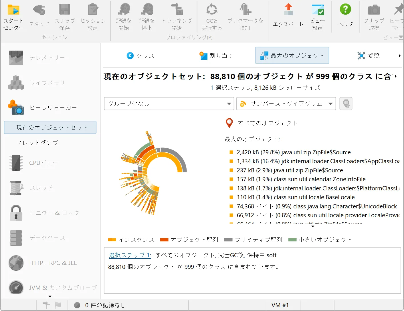
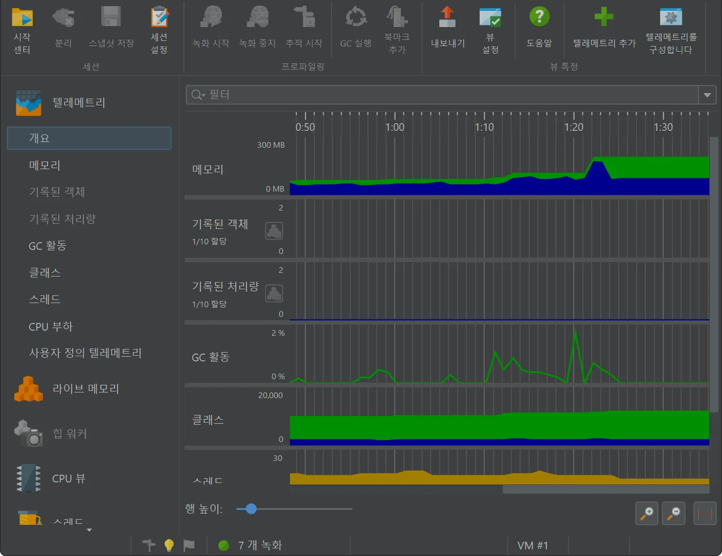
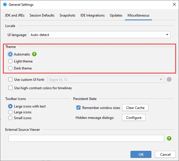
JProfiler has a new UI with a modern visual appearance and new icons. We hope you like it! We have light and dark themes.
You can see screenshots of them by toggling the dark mode switch at the top of this page.
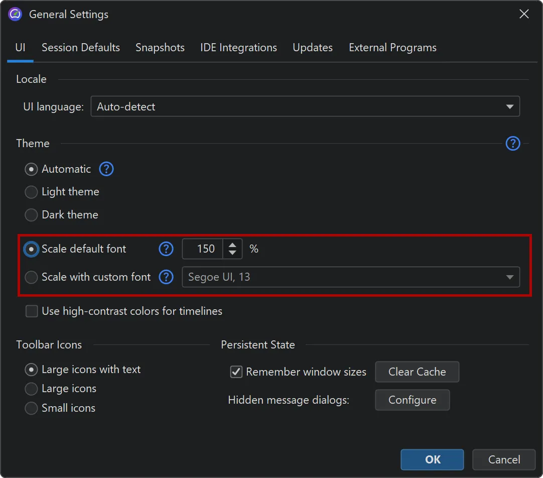
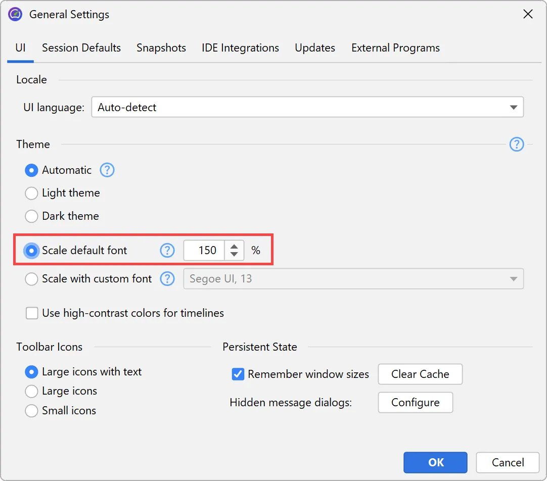
In addition, the UI is now fully scalable. In the general settings, you can either set a scale factor as a percentage, or set a
custom UI font with an arbitrary size, and the UI will be scaled accordingly.
This capability now allows the JProfiler UI to run on Linux with all OpenJDK variants and for all HiDPI resolutions. Previously, only
the JetBrains runtime was supported on Linux with HiDPI resolutions.
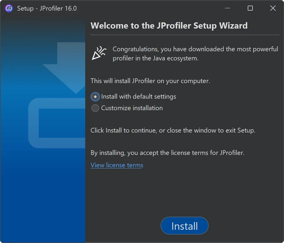
The JProfiler installer has been modernized, and its default execution mode has been streamlined. By default, no admin privileges are requested
unless you choose to install for all users in its customized execution mode.
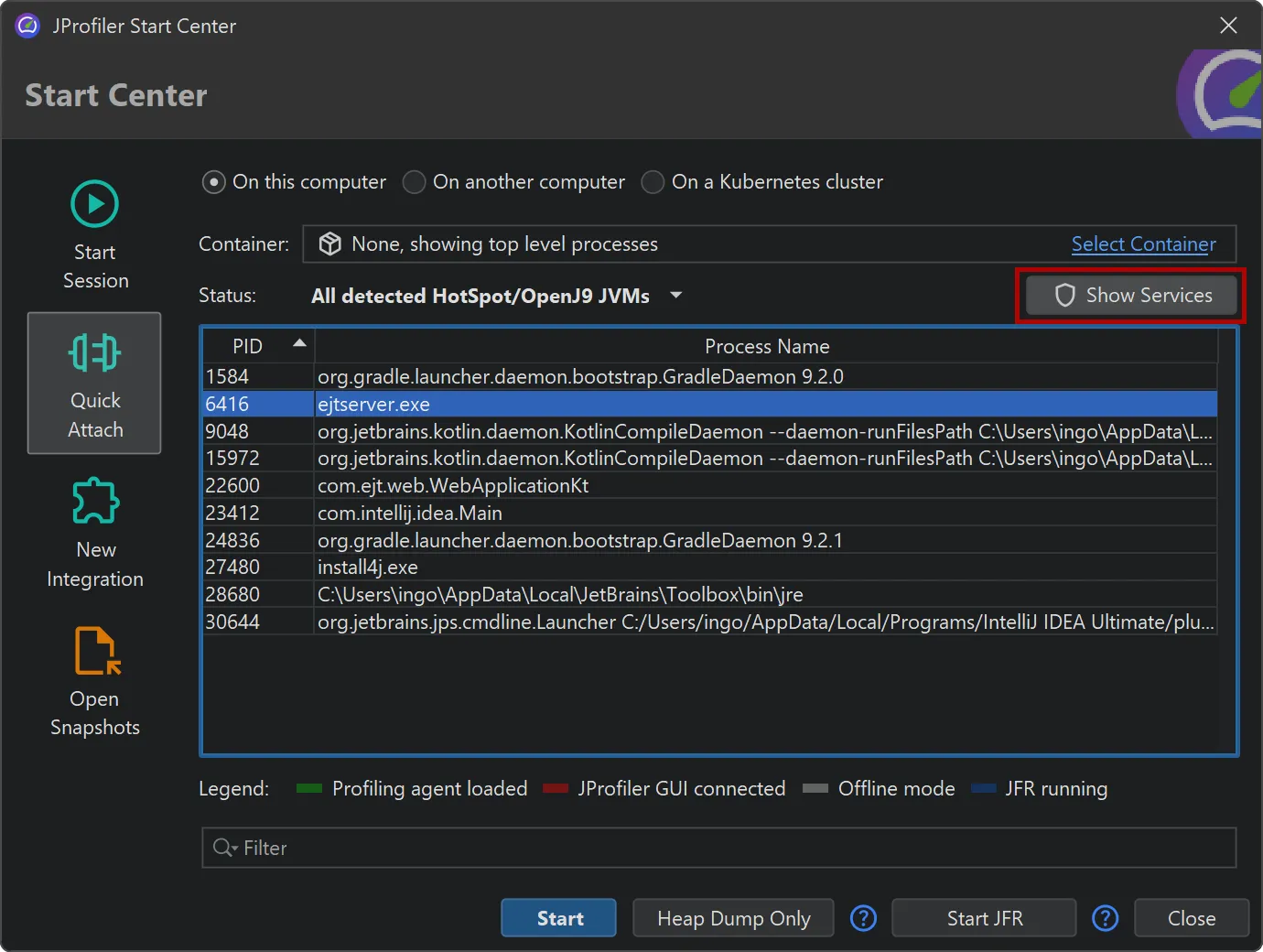
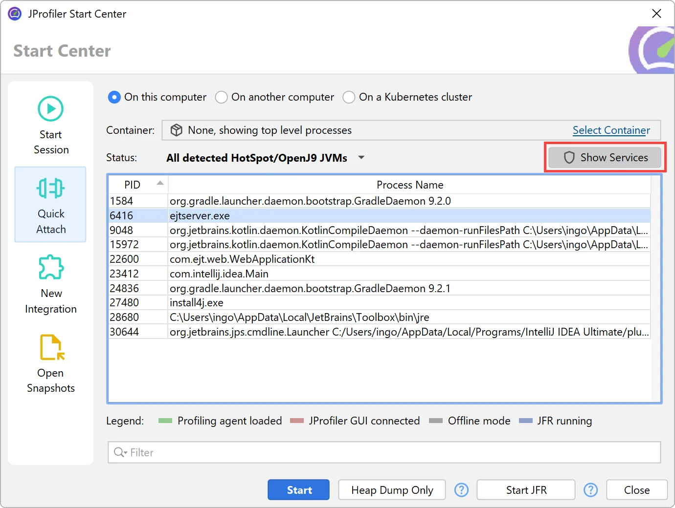
As a related enhancement, it is now possible to attach to Windows processes running as other users, even if JProfiler is not installed
in a directory that is readable by those processes. This is especially important for attaching to Windows services.
JProfiler's probe event recording has been reimplemented. This brings scalability to many millions of events and many new features.
When probes were introduced in JProfiler 7, the focus was on cumulative data, like hot spots and telemetries. Single events were available
as a tool for debugging problems, but they were all held in memory, so they were limited to relatively low event counts.
However, keeping all events enables advanced filtering that is impossible to achieve using aggregate data alone. The new file-based
backend supports high-throughput recording, enabling complex queries across massive event sets that were previously impossible to
process.
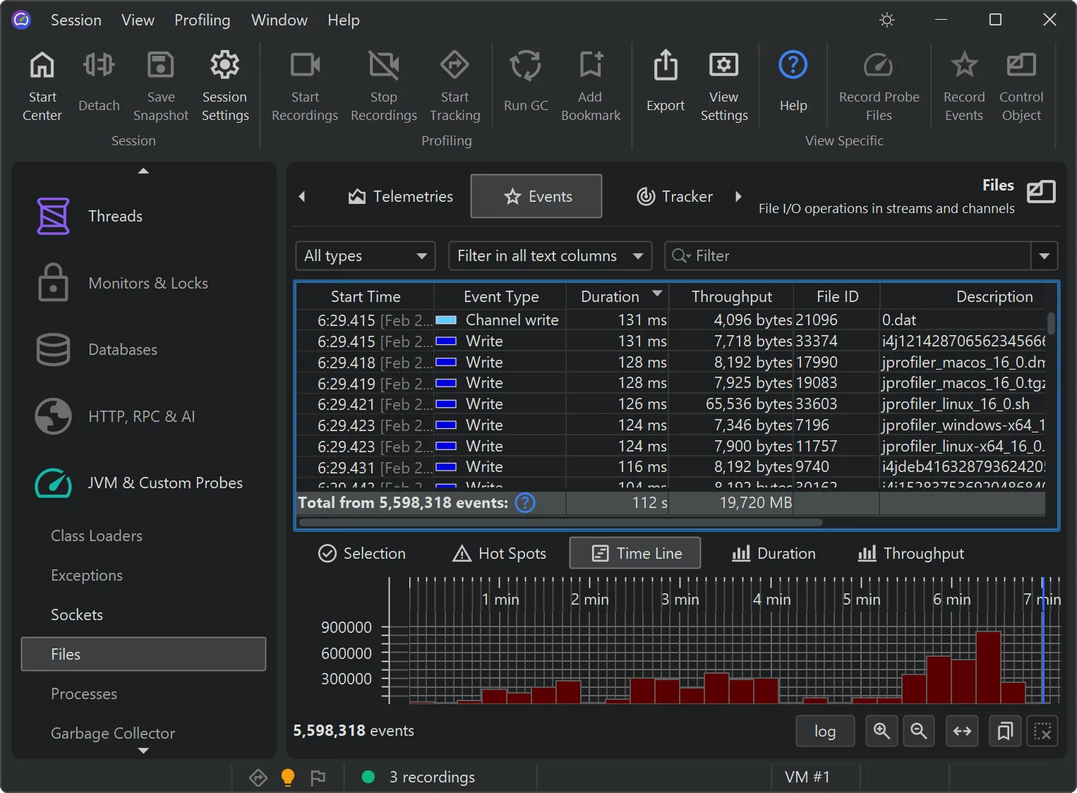
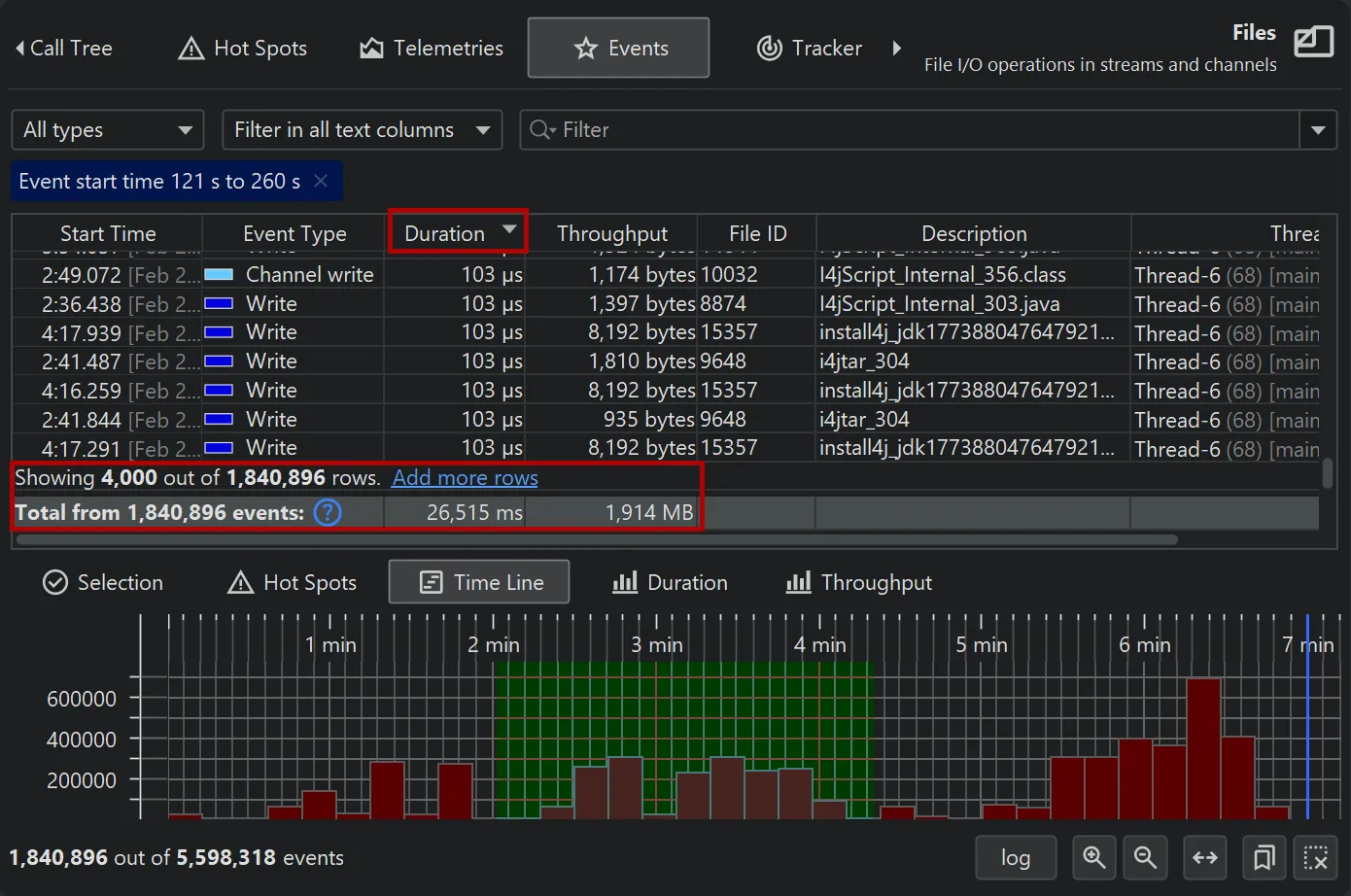
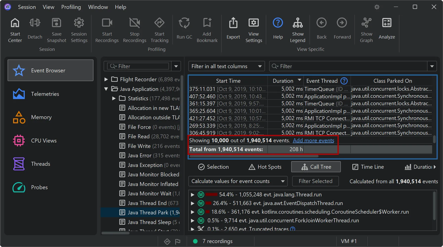
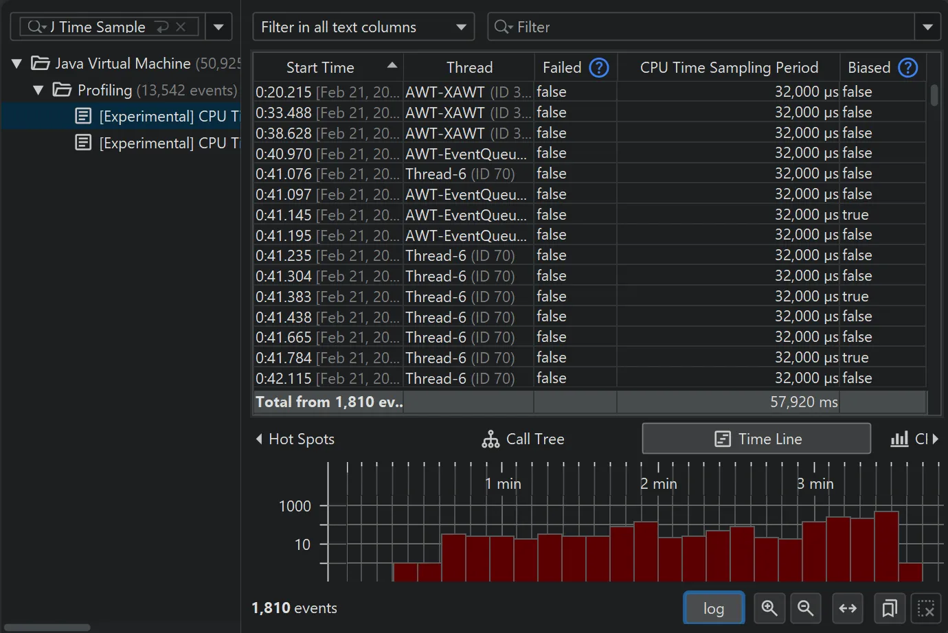
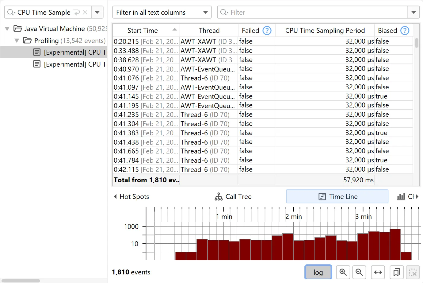
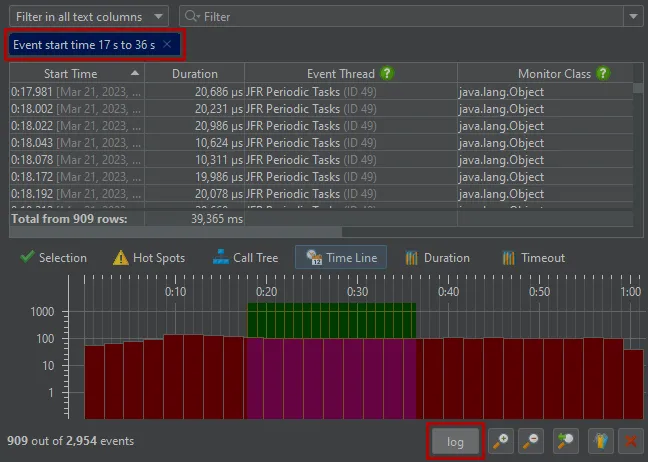
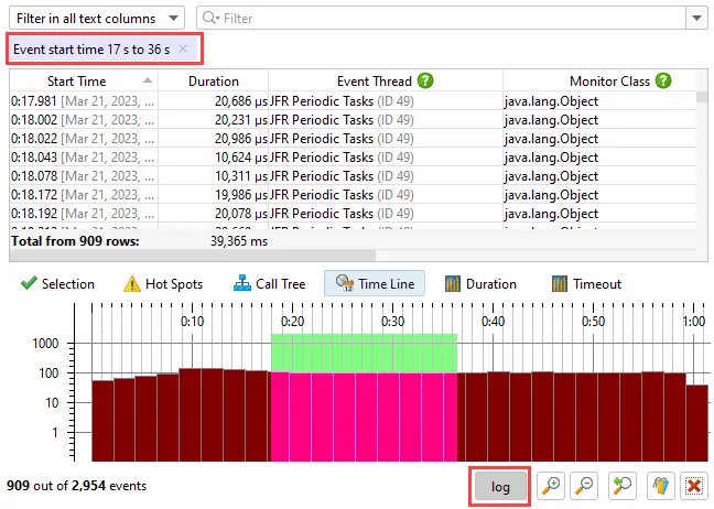
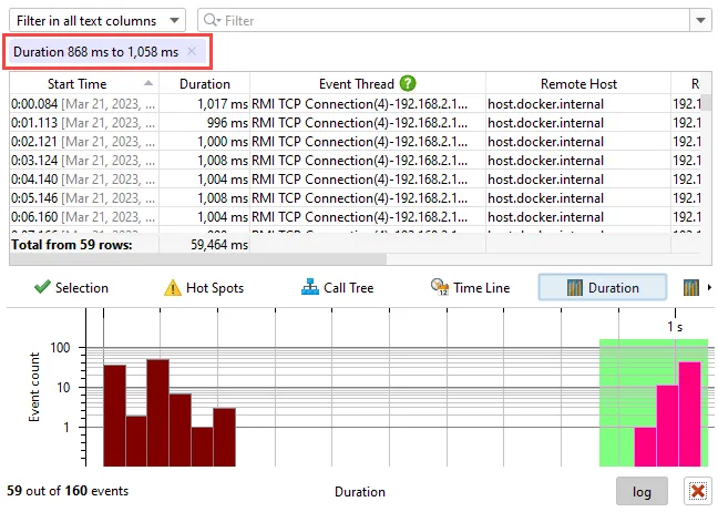
The new timeline tab at the bottom of the events view shows a histogram of all recorded events and allows you to select a time
range for filtering.
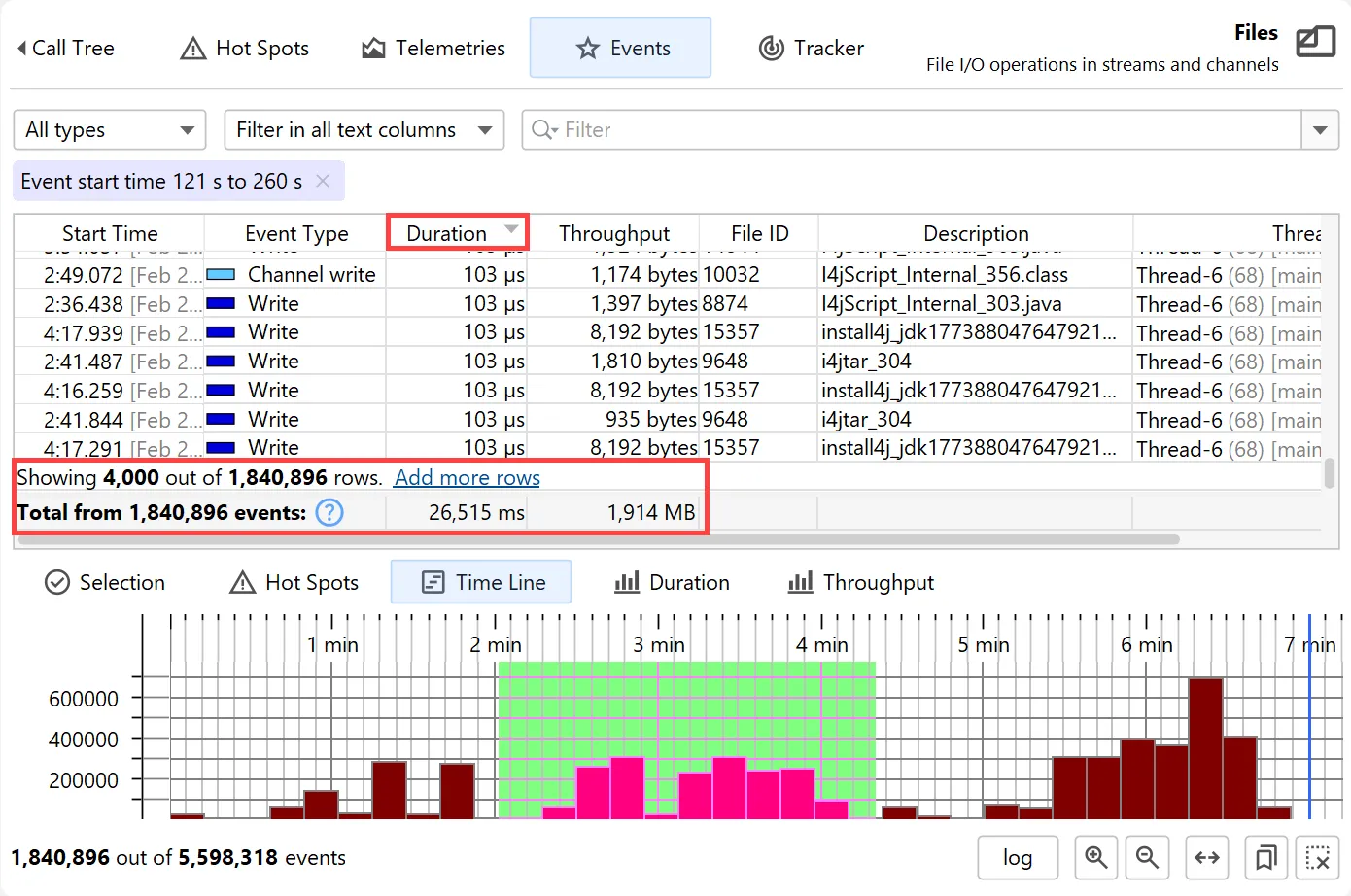
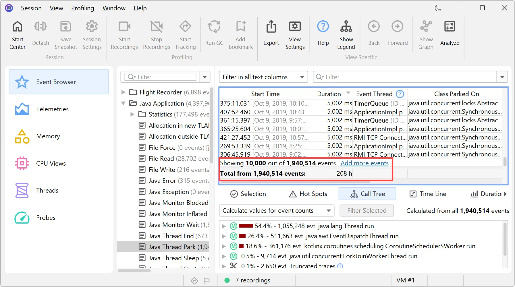
While the table only shows a limited number of events, you can add more events when scrolling to the bottom. When sorting by a column,
the entire set of filtered events is considered, not just the currently visible rows.
Totals in the table are also calculated for the entire set of filtered events.
The lower "Hot Spots" tab contains a CPU hot spots view, a probe hot spots view, and a probe call tree – similar to the "Selection"
tab, but calculated for all filtered events rather than the selected rows.
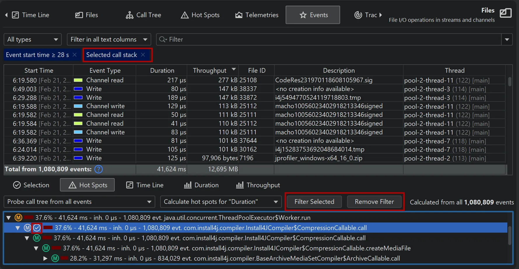
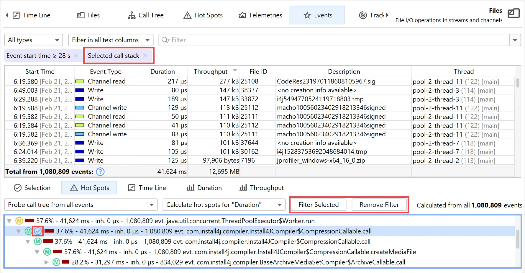
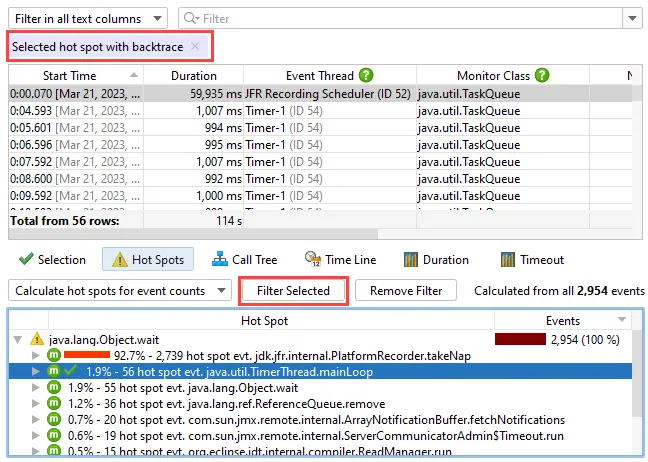
In each of these views, you can use the filter button to restrict the displayed events for the main event table and all other views
at the bottom. Below you can see a call stack filter in the probe call tree where the filtered node is marked with a filter icon.
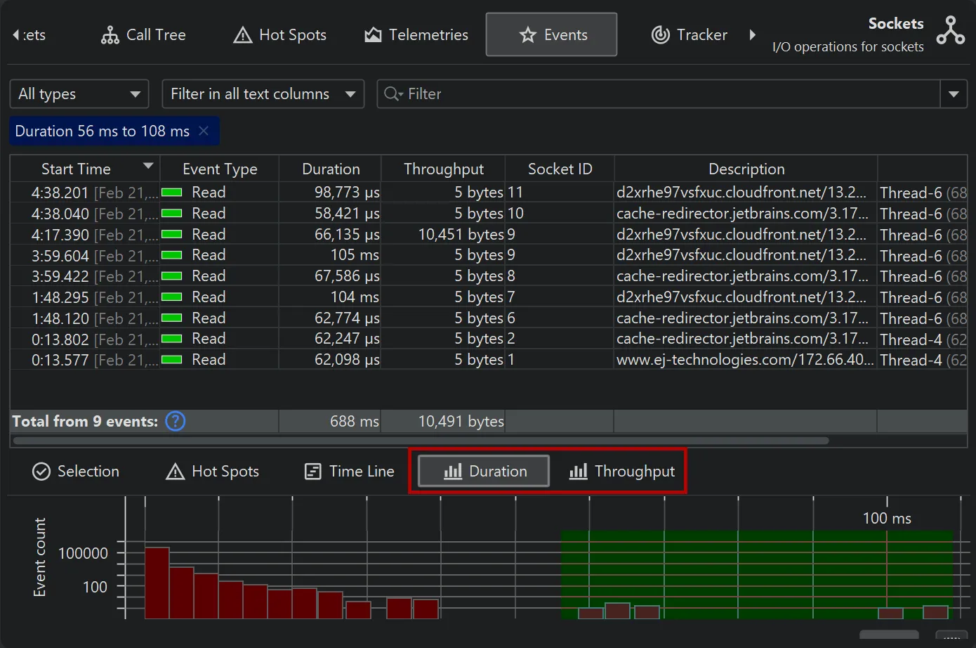
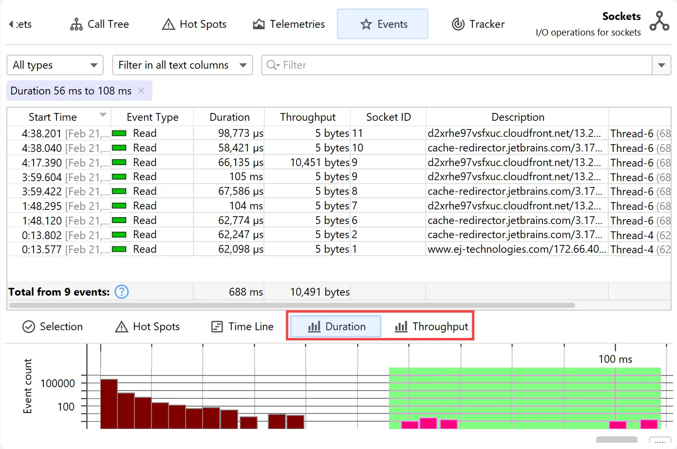
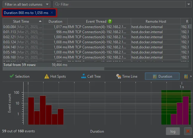
Depending on the measurements performed by a probe, additional histogram views are available at the bottom. For the "Files" and
the "Sockets" probes these are "Duration" and "Throughput".
Histograms can be shown with a logarithmic y-axis and support filtering by dragging a range with the mouse.
Finally, smart column management in the events view has been implemented. Based on the width of all columns and the available
viewport width, JProfiler decides whether to fit the columns into the viewport or activate horizontal scrolling. Resizing columns manually
disables the "fit-to-viewport" mode, which automatically reactivates if the total table width becomes smaller than the viewport.
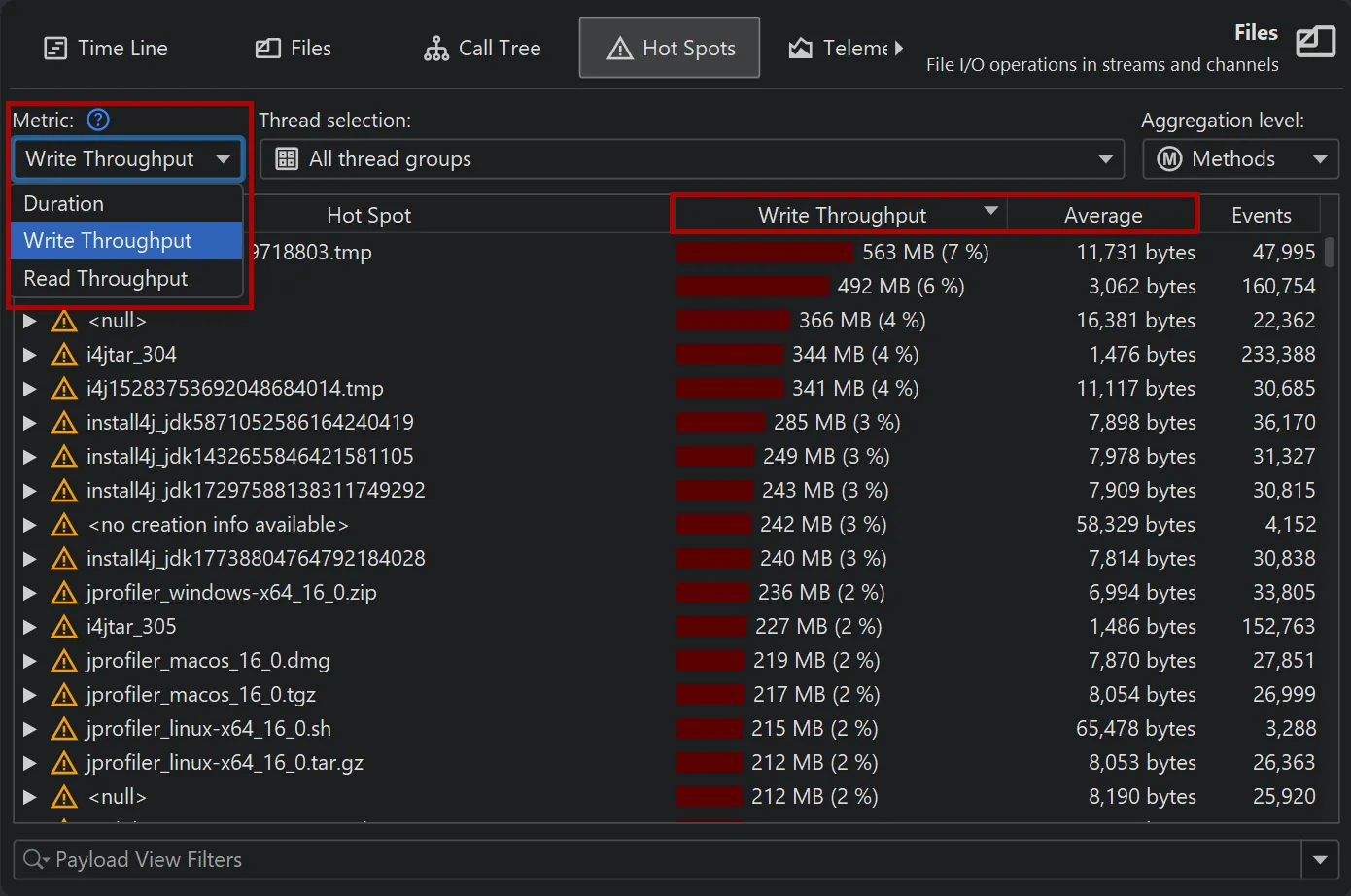
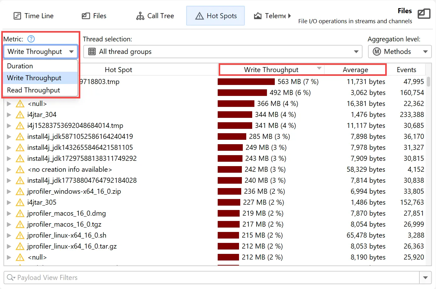
The probe call tree and probe hot spots views now have a metric selector if a probe has additional measurements beyond
event duration. For example, the "Files" and the "Sockets" probes also offer "Read Throughput" and "Write Throughput".
Selecting one of the throughput metrics automatically restricts the view to "Read" or "Write" events, respectively.
Changing the metric recalculates hot spots and updates the hot paths in the probe call tree.
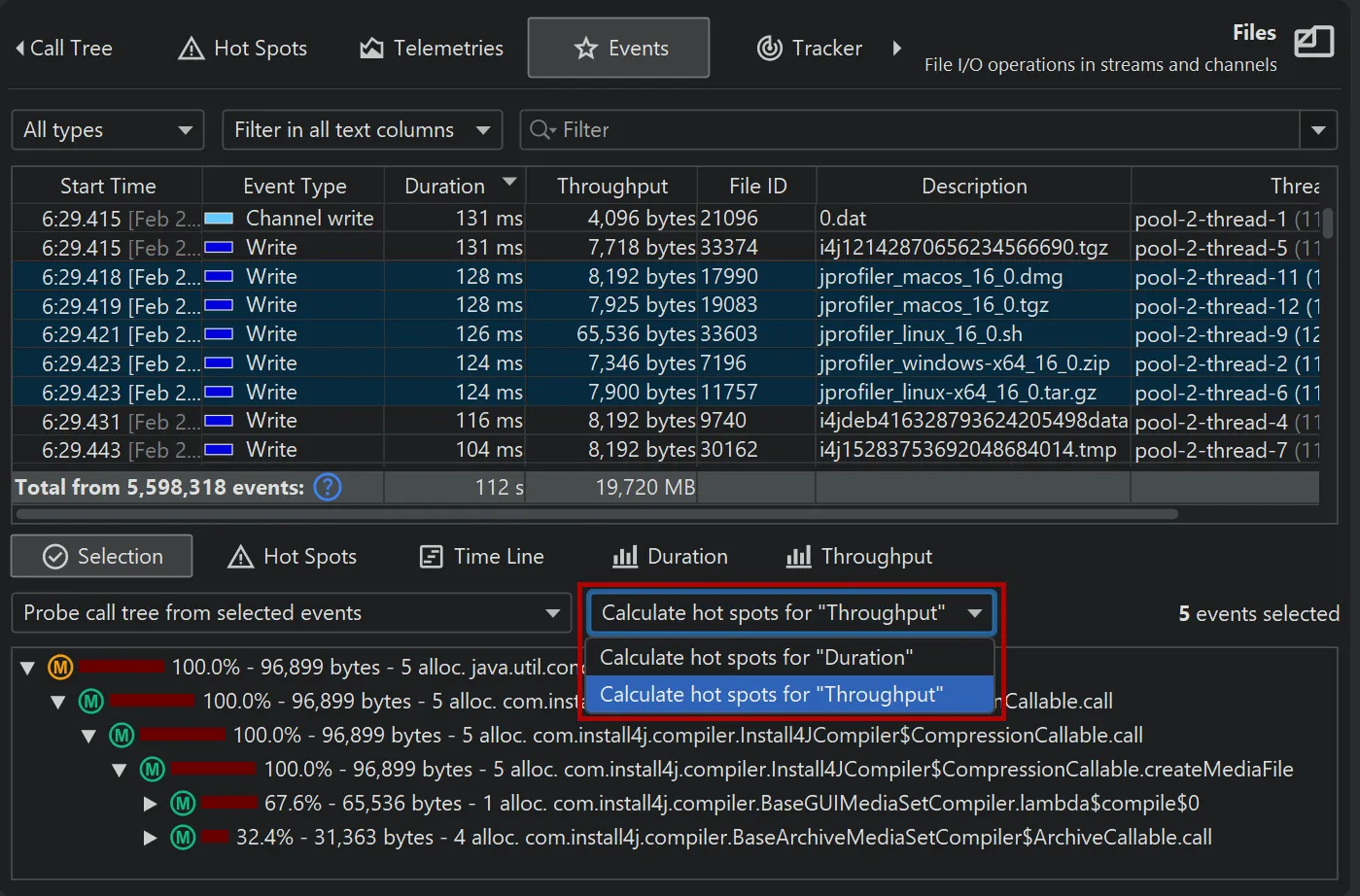
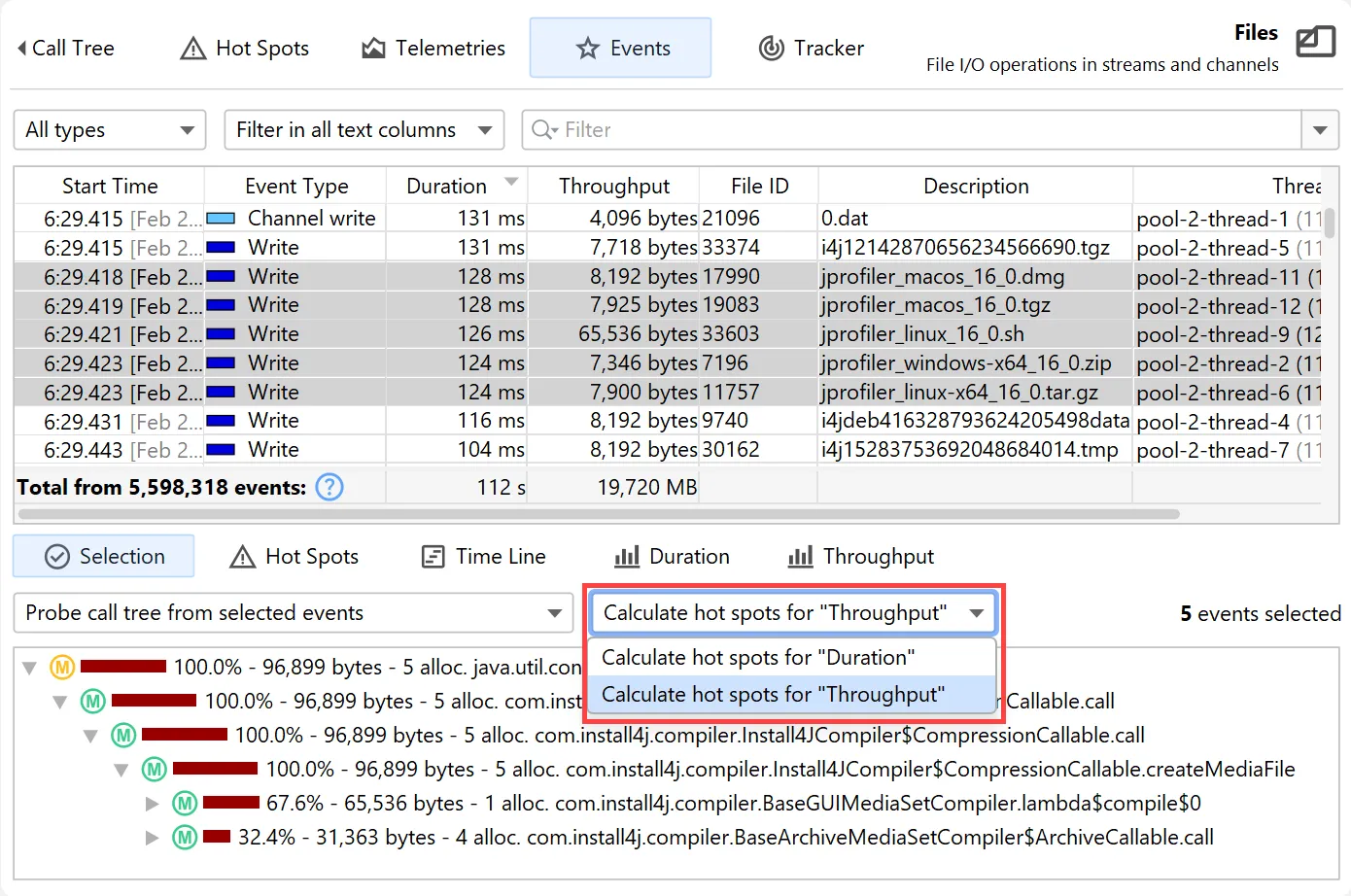
Metric selectors are now also available on the "Selection" and "Hot Spots" tabs of the probe events view. Since "Read" and "Write"
events can be filtered separately in the events view, there is a single combined "Throughput" measurement.
JProfiler 16 delivers many improvements for JFR support.
- Responsiveness in the event browser for large event counts has been improved by pre-calculating the data in the lower views.
-
Previous versions of JProfiler only handled a maximum number of events in the event table. You can now load additional events by scrolling
to the bottom. Additionally, when sorting the table, all filtered events are considered rather than just the visible subset.
- The totals in the event table are now calculated for all filtered events, not just for the currently displayed ones.
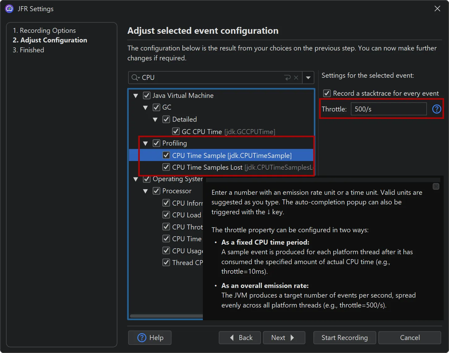
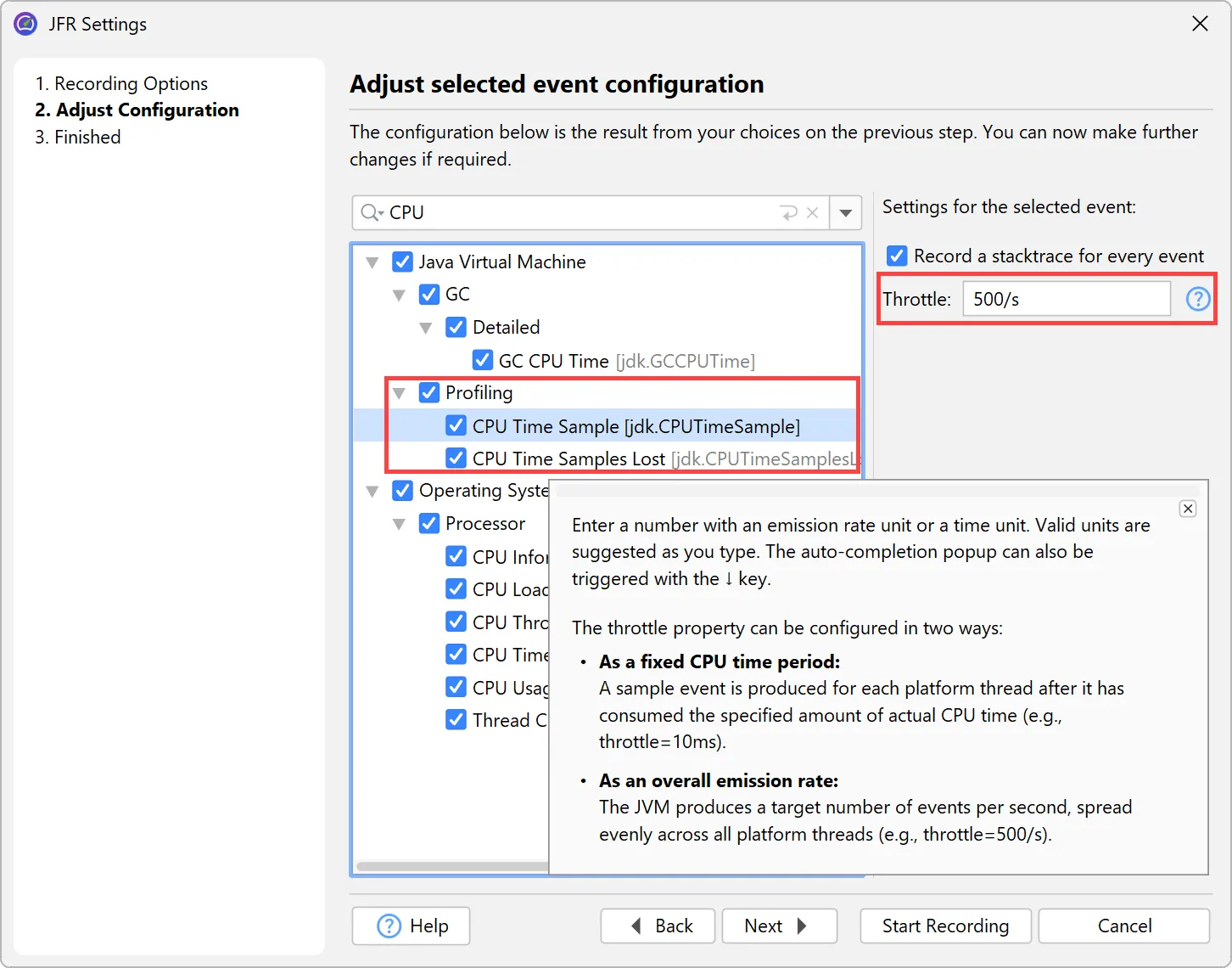
Support for throttle settings has been added in the JFR recording wizard. For example, the new jdk.CPUTimeSample event in
Java 25 is configured via throttling. You can alternatively enter a period or an emission rate with a /s unit.
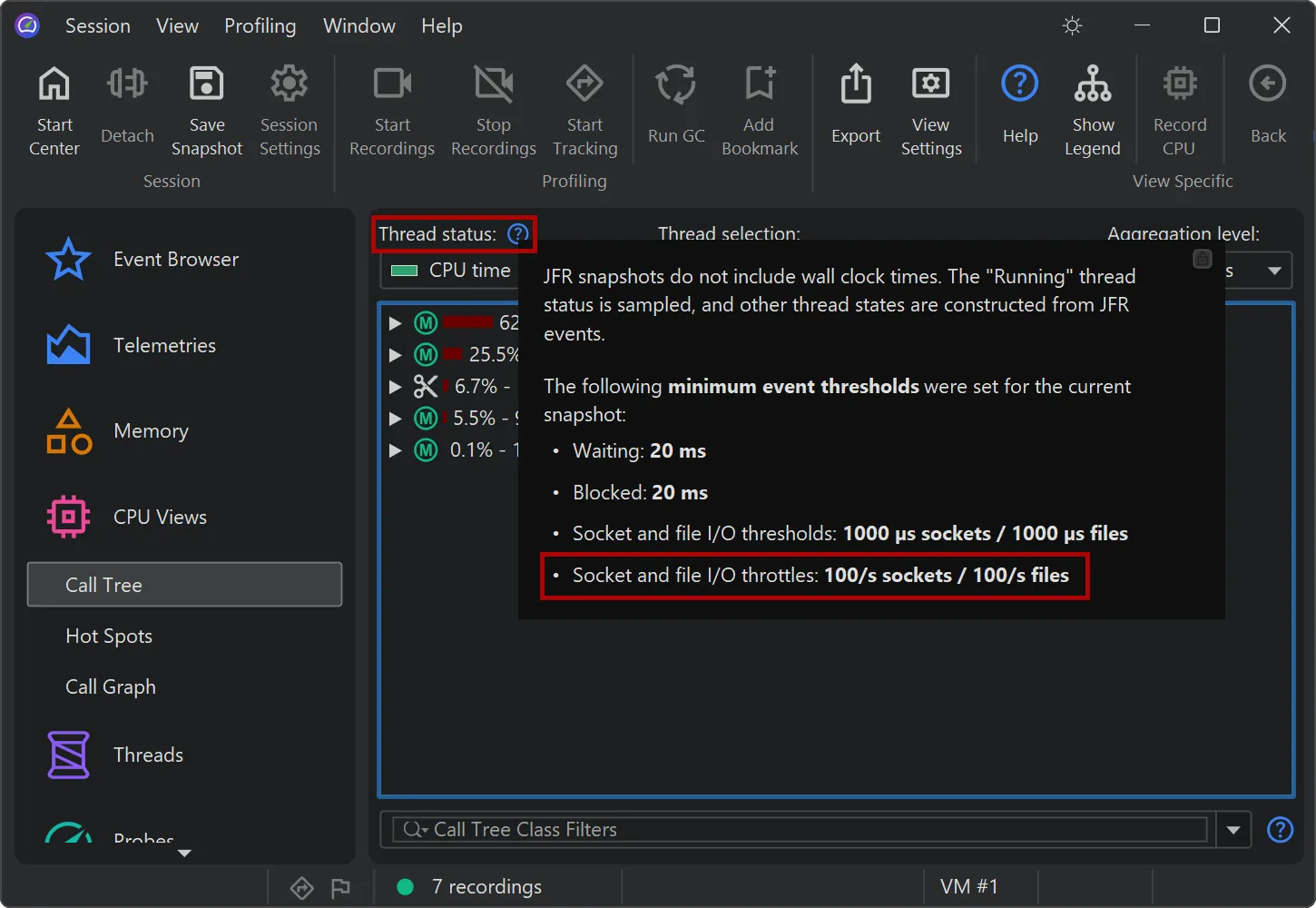
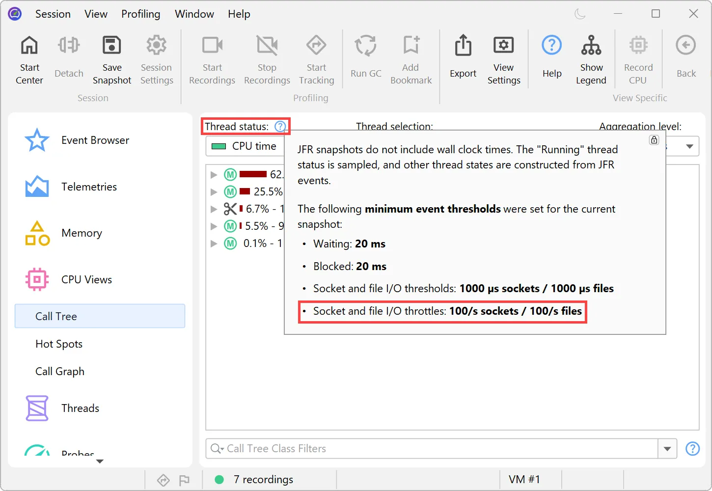
Throttle settings are also displayed in the CPU views next to the thread status selector.
For calculating data in the CPU section, the new Linux-only jdk.CPUTimeSample event (Java 25+) is now used if recorded,
instead of the older jdk.ExecutionSample event. Unlike jdk.ExecutionSample, which works on all platforms, but has
limitations in the number of threads it samples and the accuracy of CPU usage, jdk.CPUTimeSample uses CPU time events from
the Linux kernel to collect data.
With this event, CPU profiling with JFR can now provide actionable CPU metrics on production systems where loading a JVMTI agent is not
permitted.
Starting with JProfiler 16, all experimental JFR events are now shown in the event browser, such as the jdk.CPUTimeSample
event.
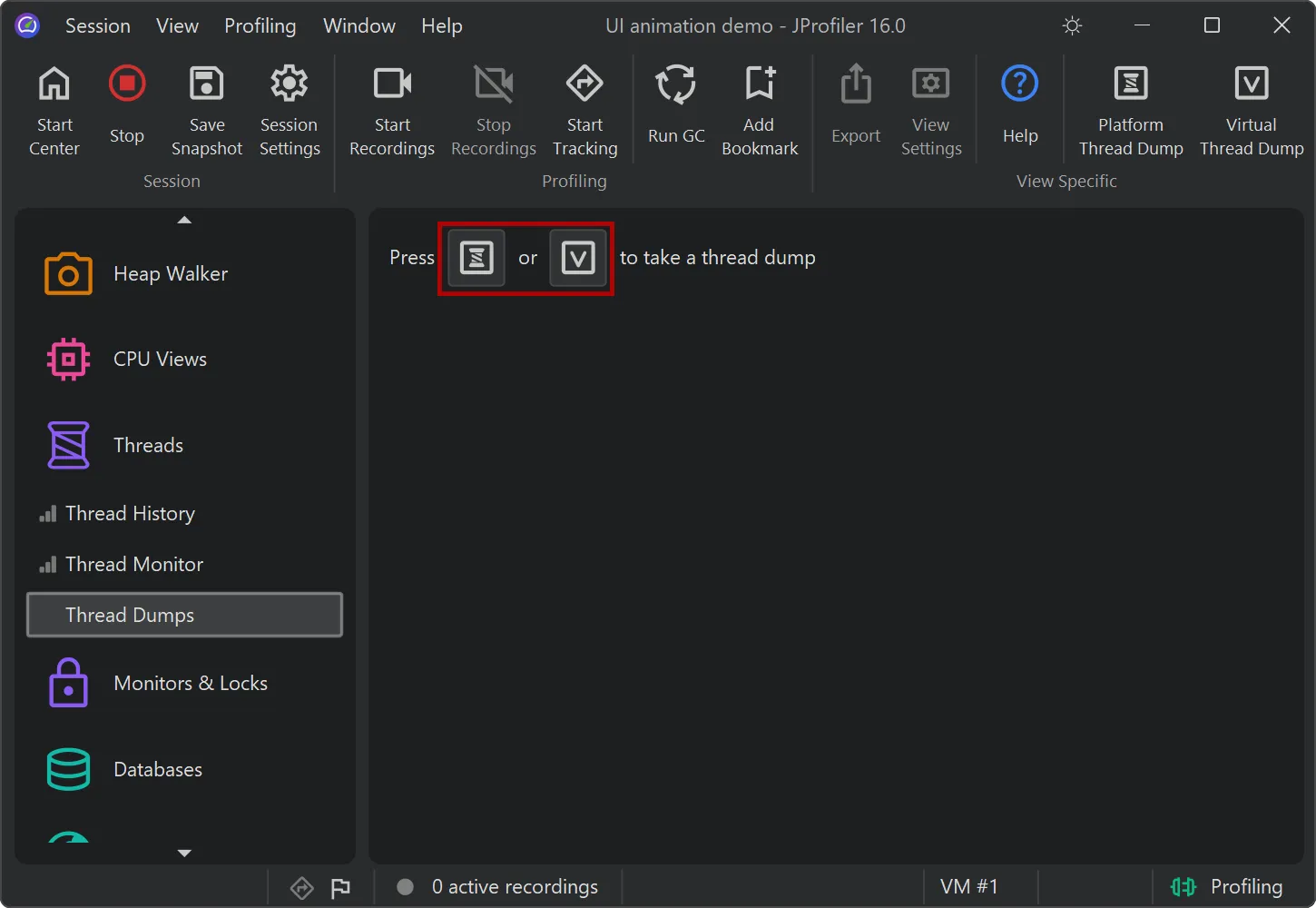
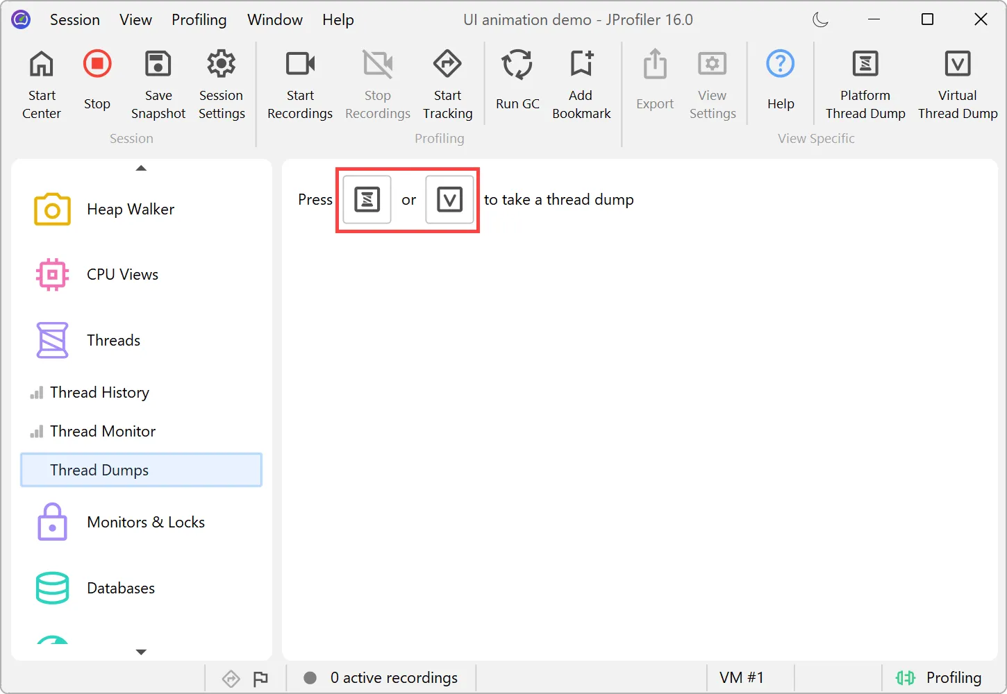
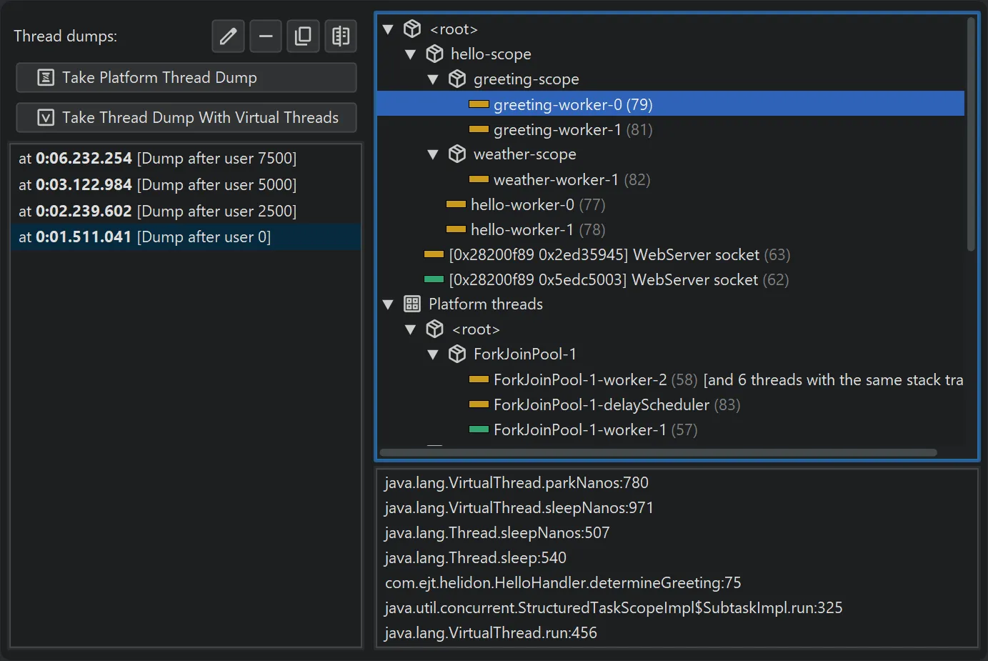
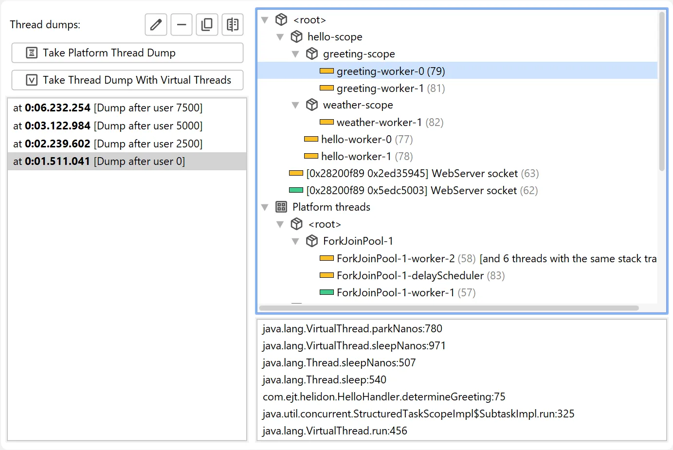
JProfiler 16 introduces support for virtual thread dumps.
The thread dumps view now features two distinct actions: one for platform thread dumps and another for virtual thread dumps.
While the virtual thread dump also includes platform threads, it is asynchronous, so synchronous platform
thread dumps are preferable when not working with virtual threads.
Virtual threads are hierarchically organized within their thread containers. This is relevant when using
structured concurrency, which is still a preview feature as of Java 25.
In structured concurrency, each scope creates a corresponding thread container. Since a dump may contain millions of virtual threads
in deeply nested containers, virtual thread dumps can be significantly larger than platform thread dumps.
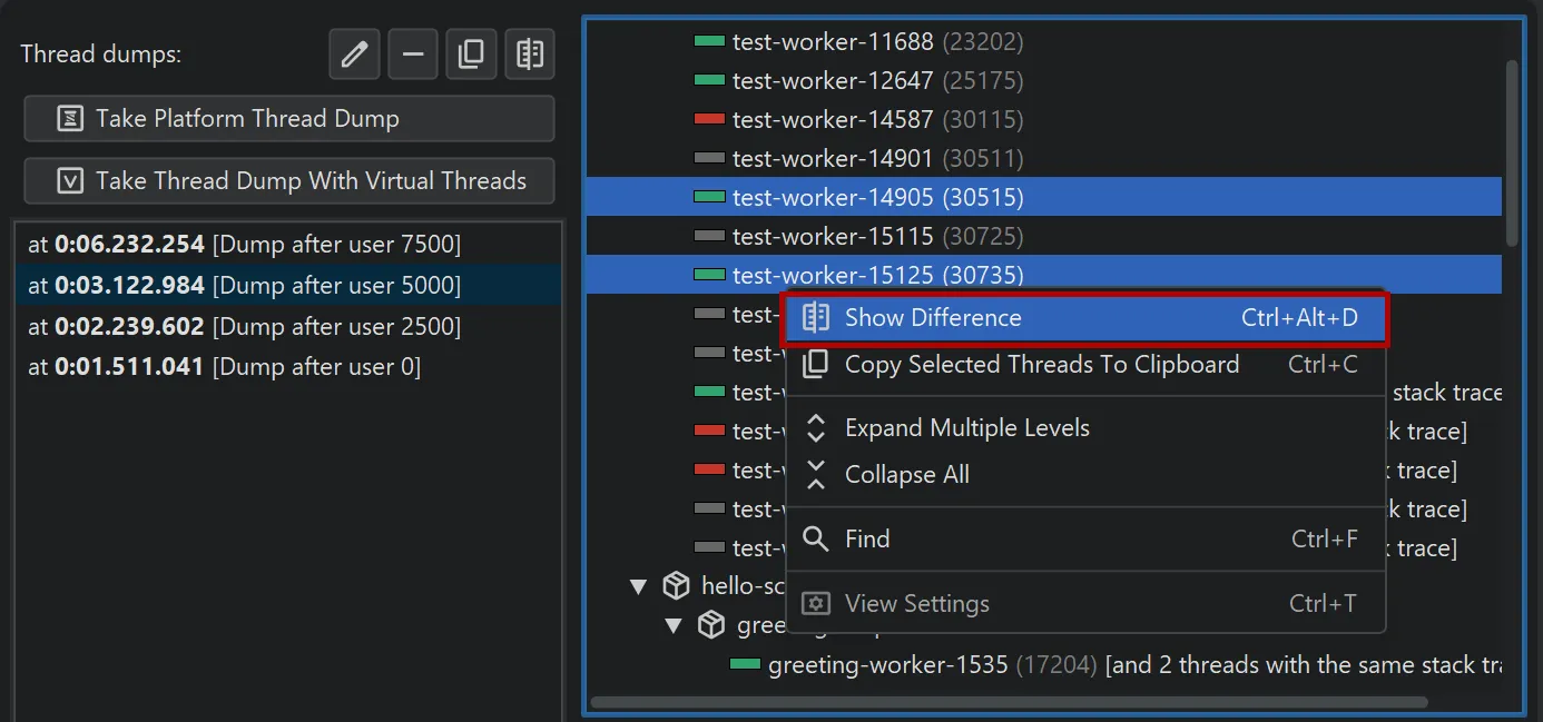
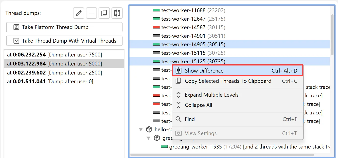
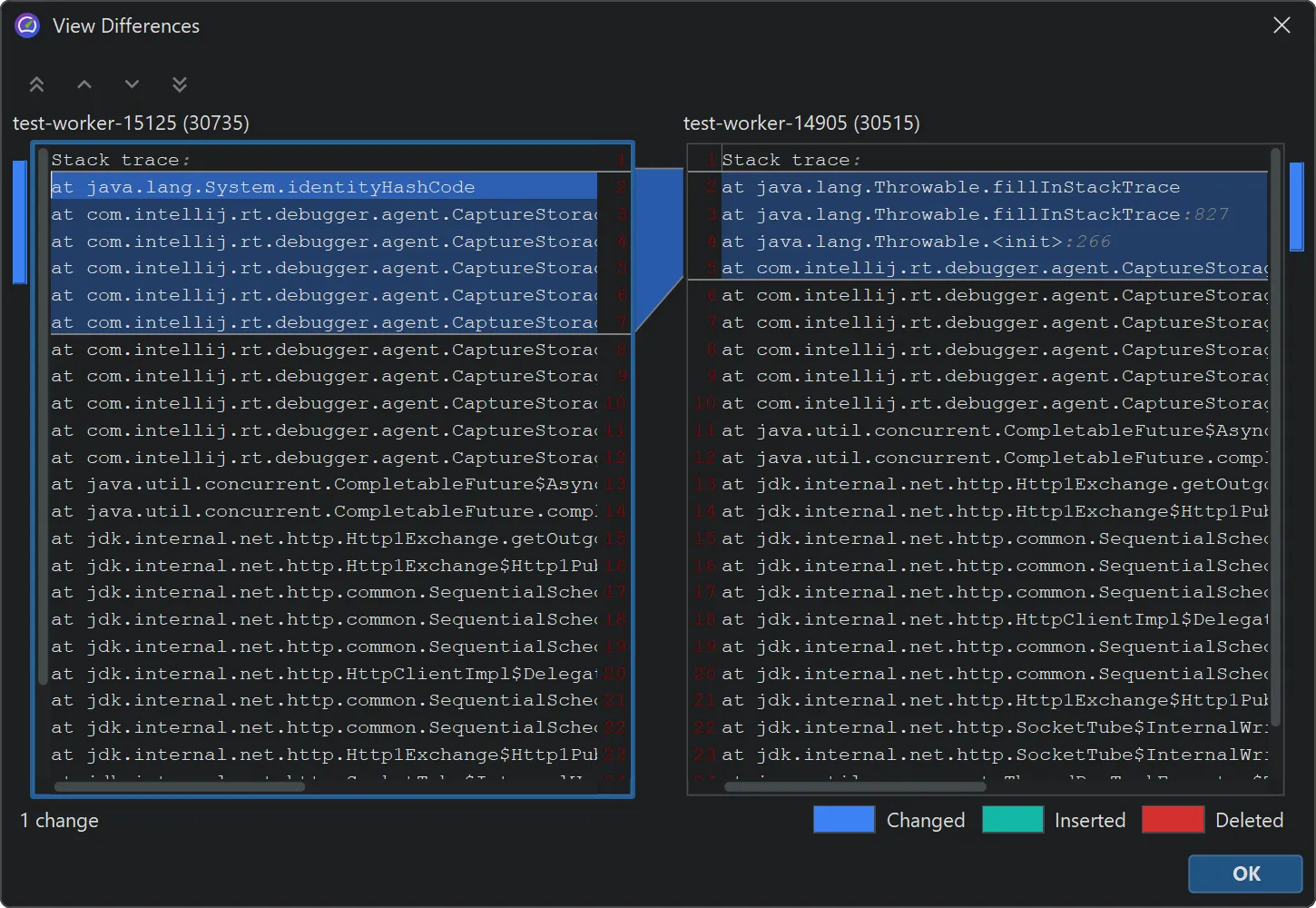
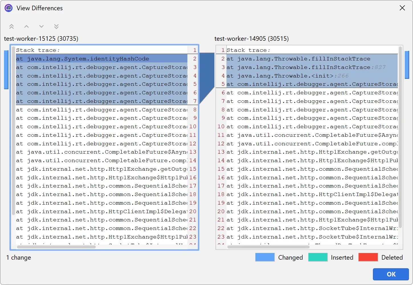
You can compare two single virtual threads or two entire thread dumps by selecting them and choosing the comparison action in the
context menu.
The comparison is shown in a diff viewer in a separate window.
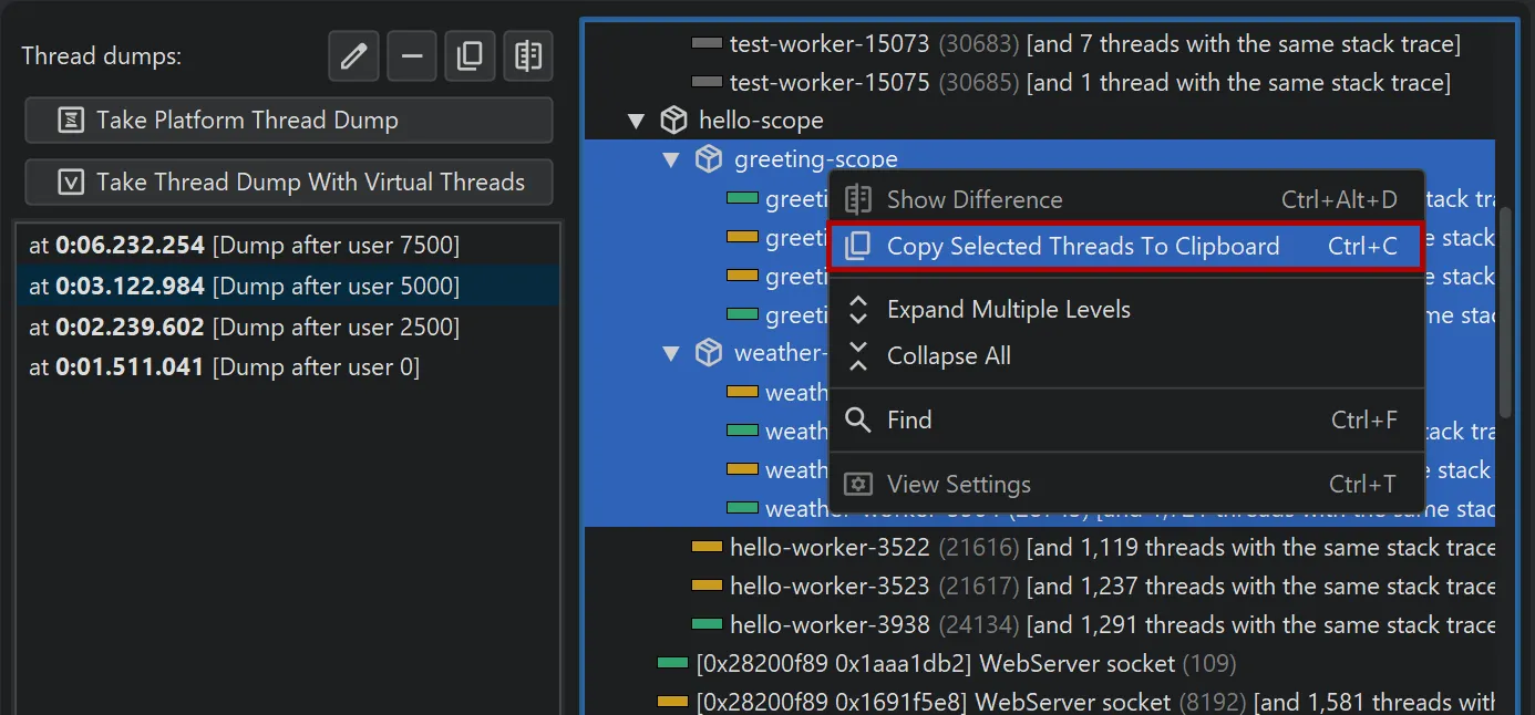
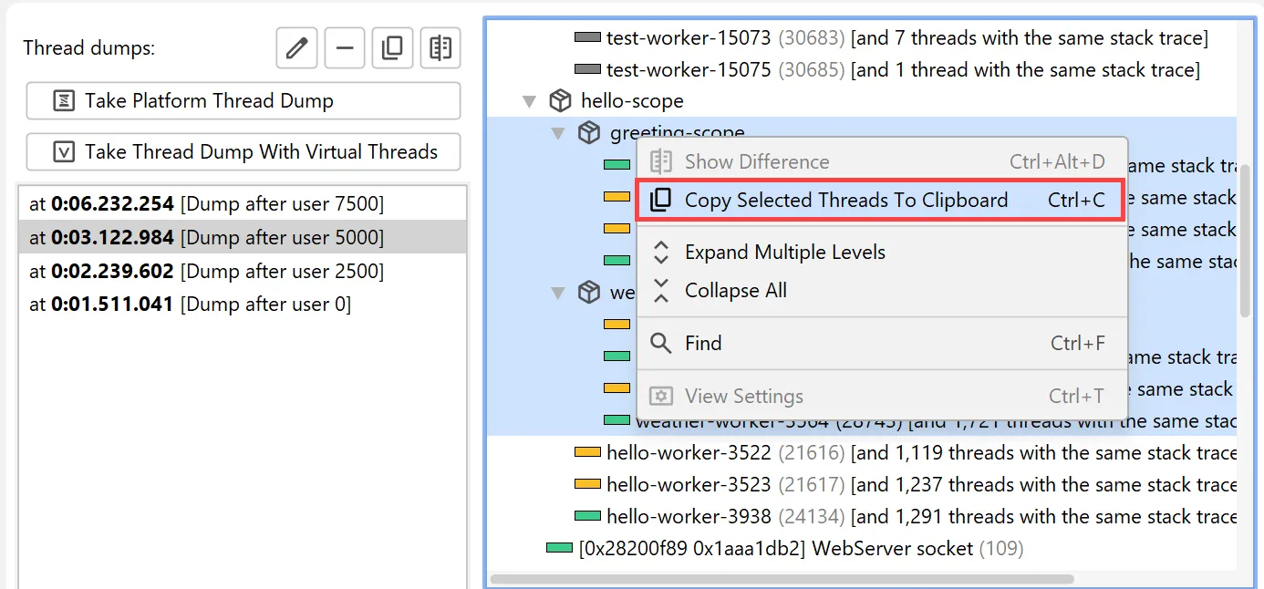
To copy single threads, multiple threads, or entire thread dumps to the clipboard, use the corresponding action in the context menu.
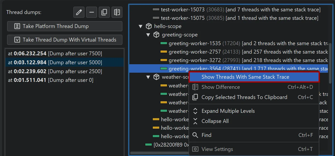
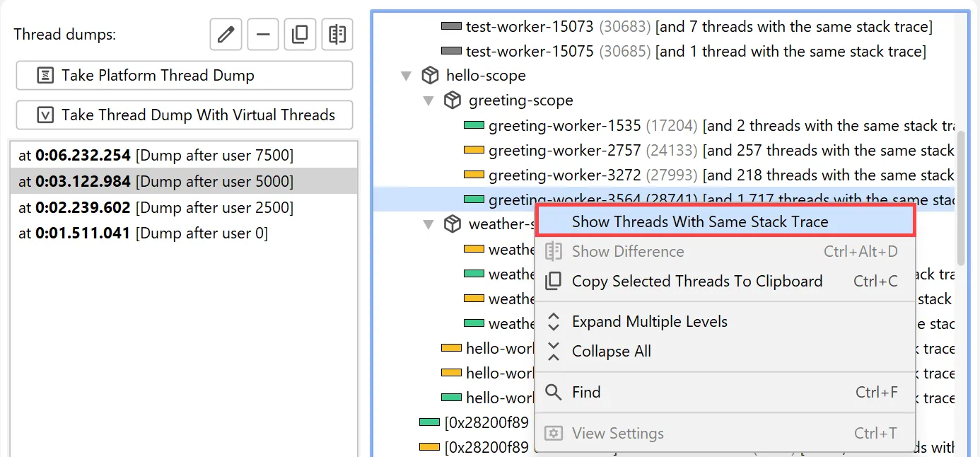
Virtual thread dumps group threads with the same stack trace in the same hierarchical position into a single node.
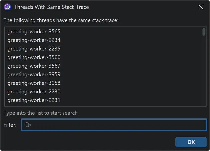
The context menu contains an action to show all grouped thread names.
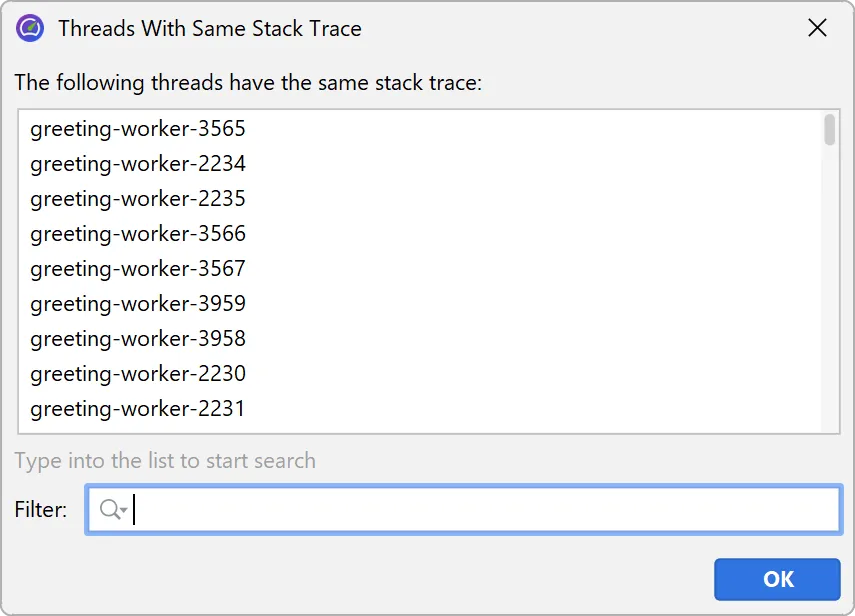
The names of grouped threads are displayed in a separate window where you can filter for thread names of interest.
Thread grouping is also supported for platform thread dumps.
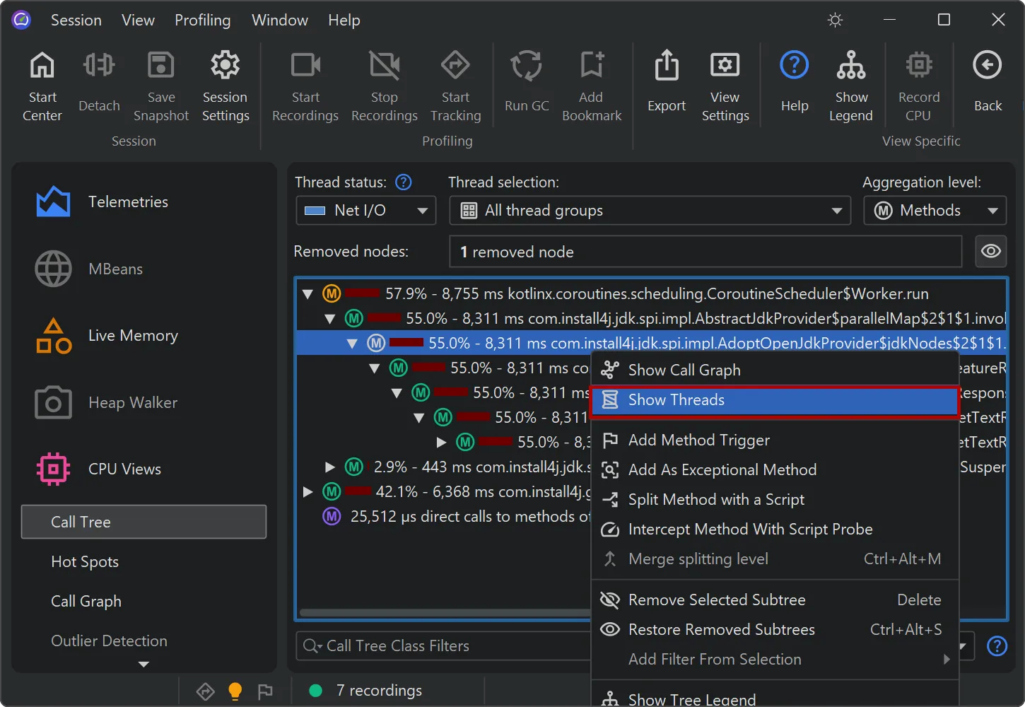
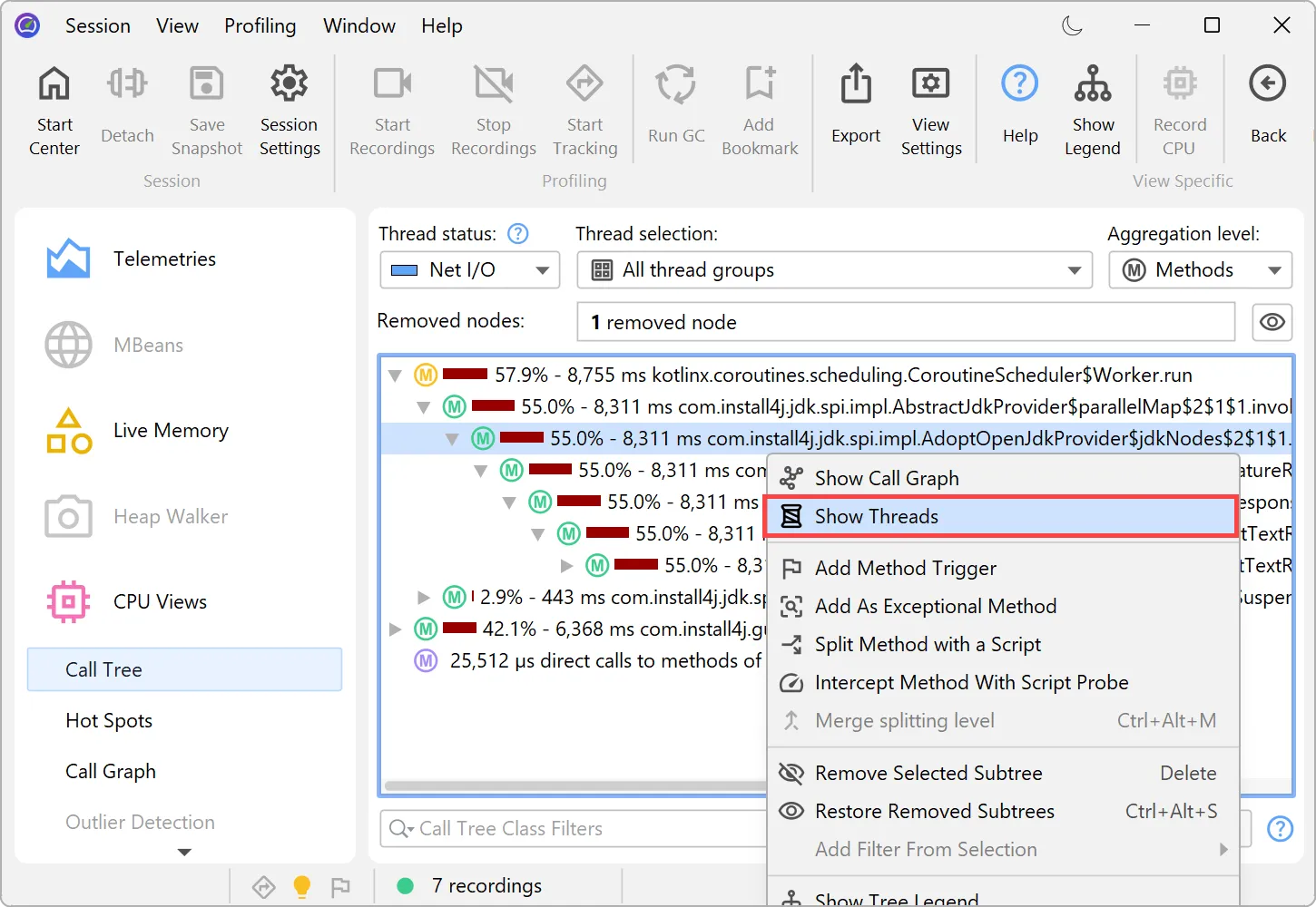
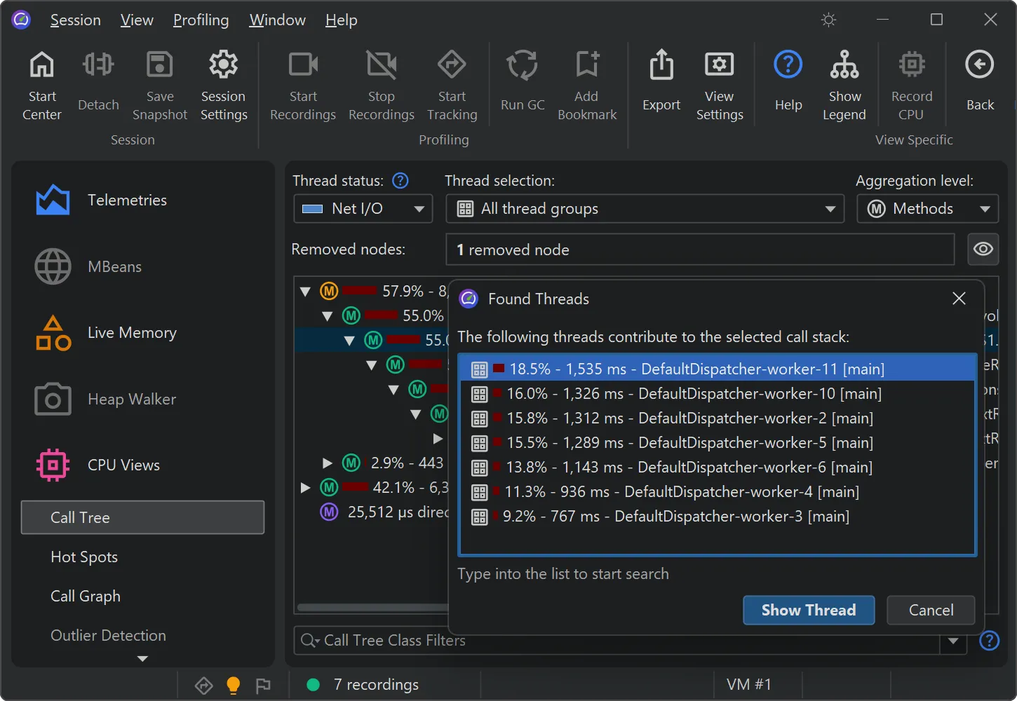
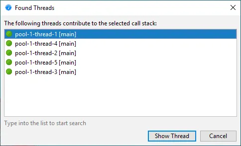
You can now analyze the contribution of single threads in a cumulative call tree. In the call tree view,
select "Show Threads" from the context menu to calculate this data for the selected node.
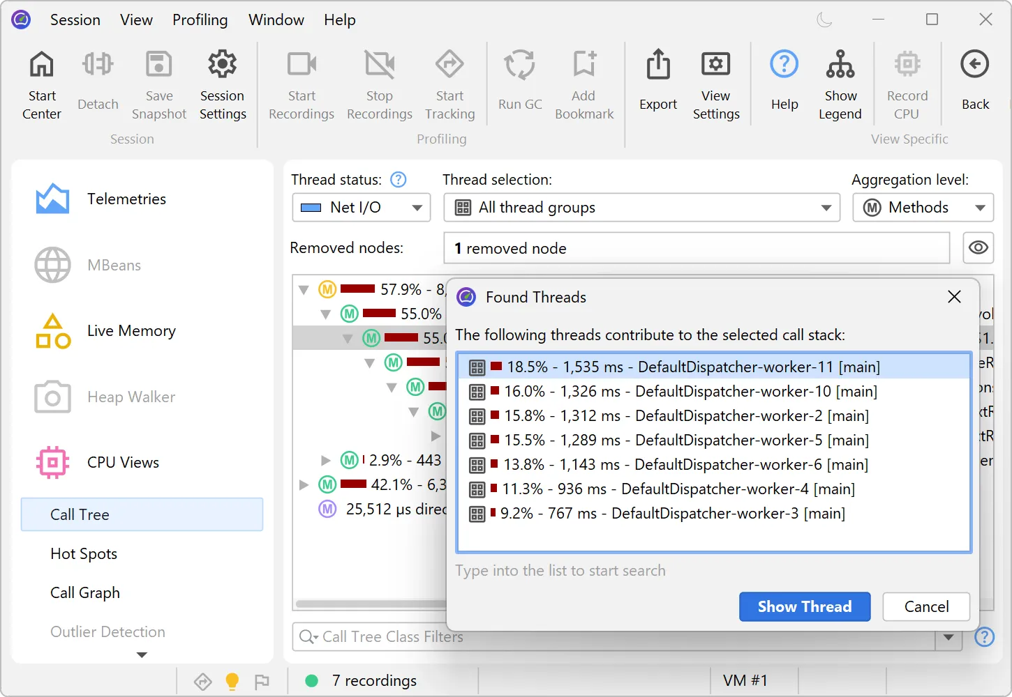
A separate dialog with a percentage breakdown of all contributing threads is shown. You can optionally select one thread
and switch to the call tree for that thread in the call tree view.
The feature helps identify thread-specific performance issues. For example, you may want to isolate a misbehaving thread from a thread pool.
The node detail dialog was improved in several ways.
The node detail dialog is an important tool to display more information for selected elements and is available from the "View" menu or
the context menu.
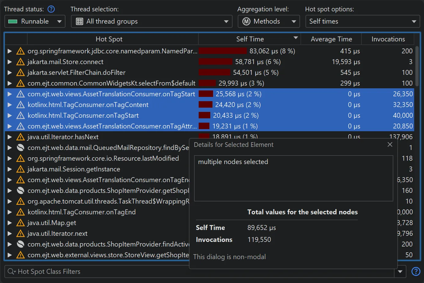
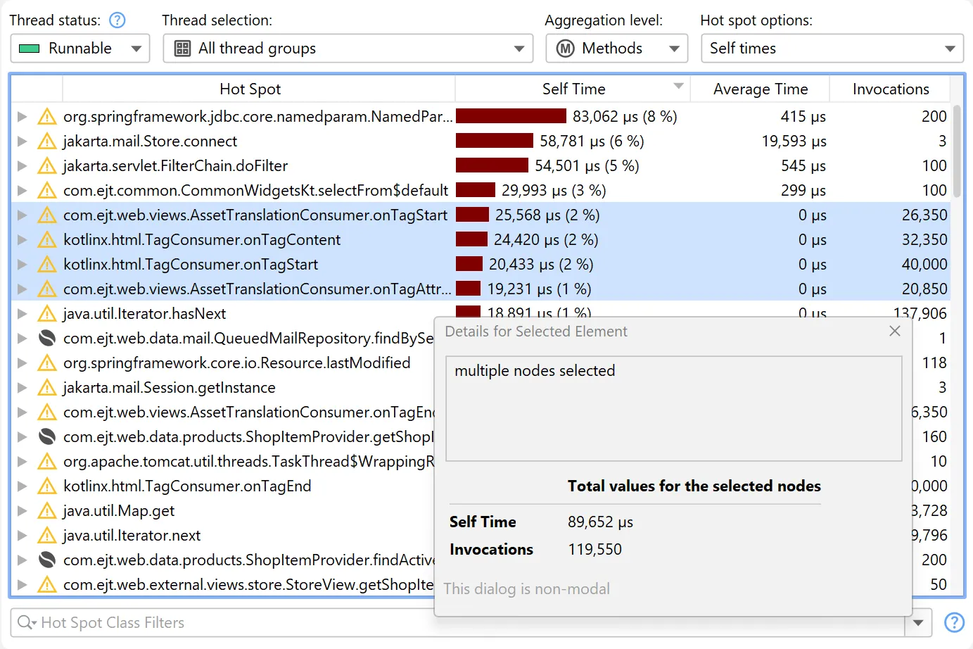
When selecting multiple nodes in hot spots views, cumulative statistics for the selection are now displayed.
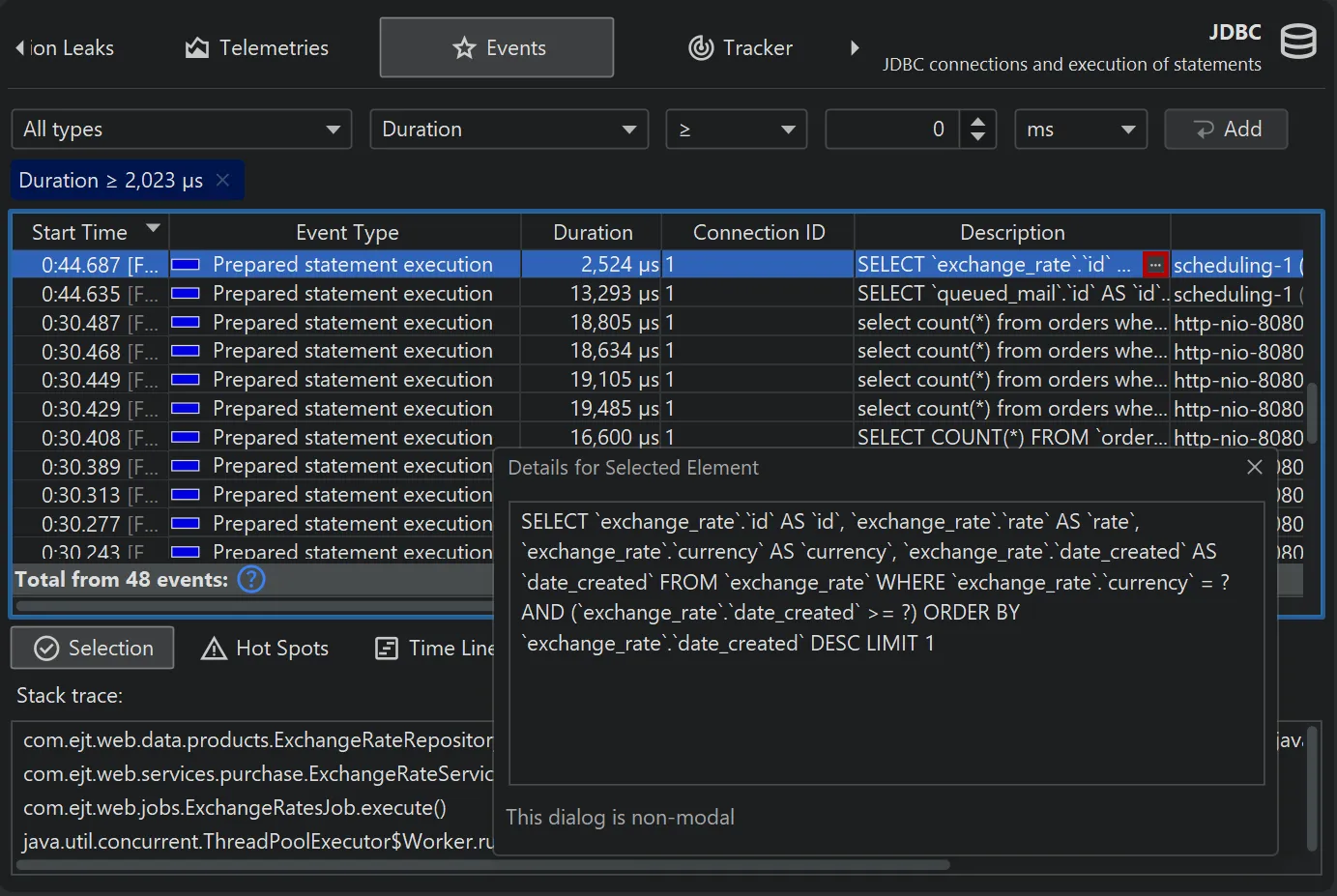
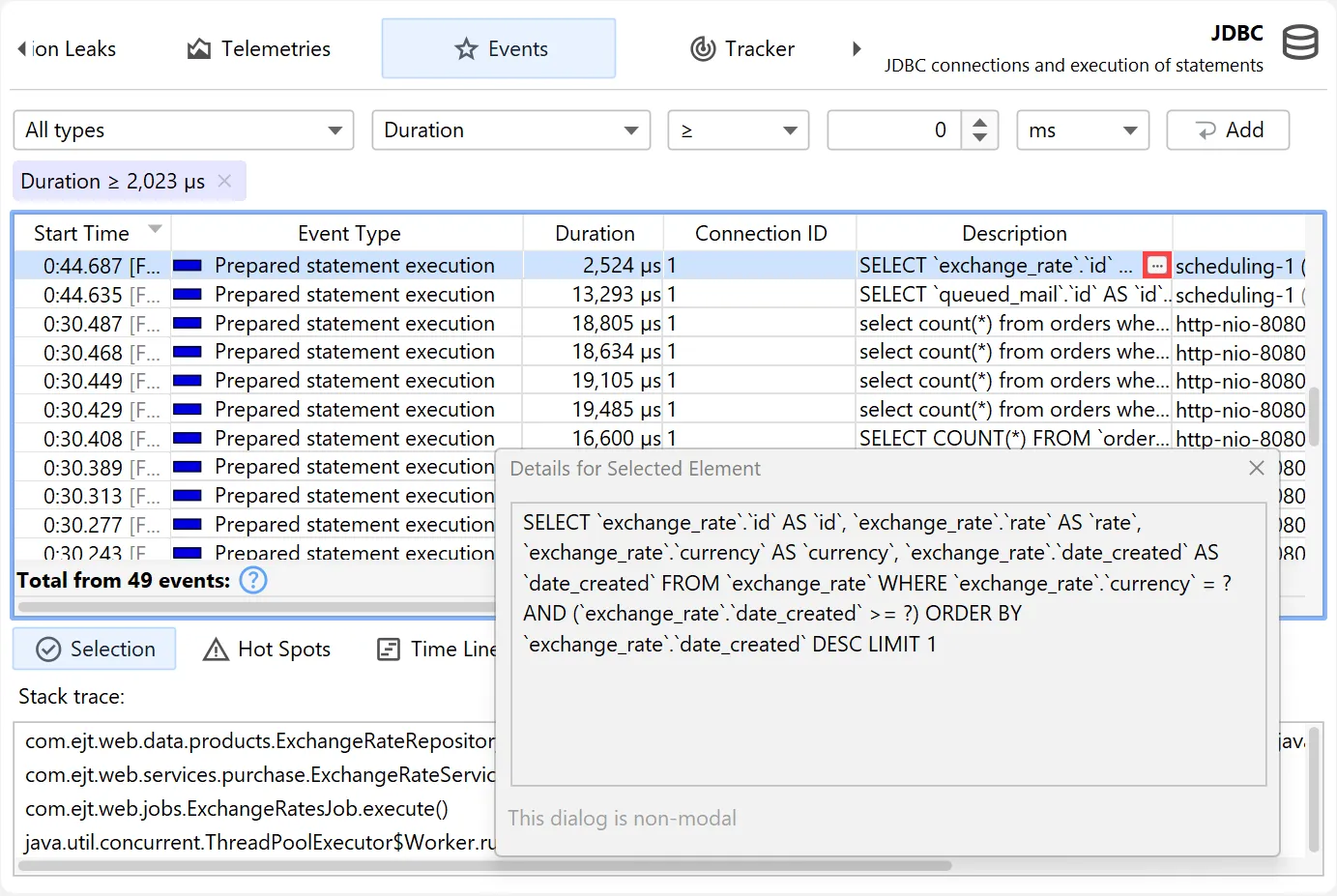
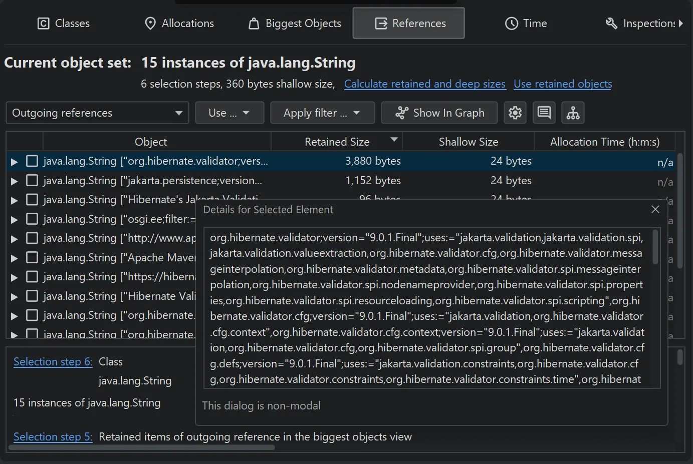
Many tables in JProfiler have columns containing long text that exceeds the column width. The node detail dialog
shows the complete text in this case. Starting with JProfiler 16, there is a hover button that directly opens the node detail dialog and activates
the correct tab if there are multiple long text columns in the table.
In the heap walker, the node detail dialog now shows the full values for string values in the reference views, not just the displayed
truncated preview string.
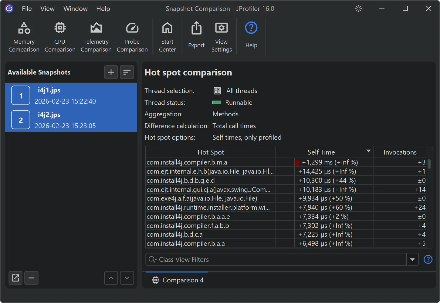
JProfiler now supports deobfuscation for snapshot comparisons.
Previously, when comparing snapshots from an obfuscated application, there was no way to deobfuscate classes and methods.
Below, you can see an example of a comparison using obfuscated names.
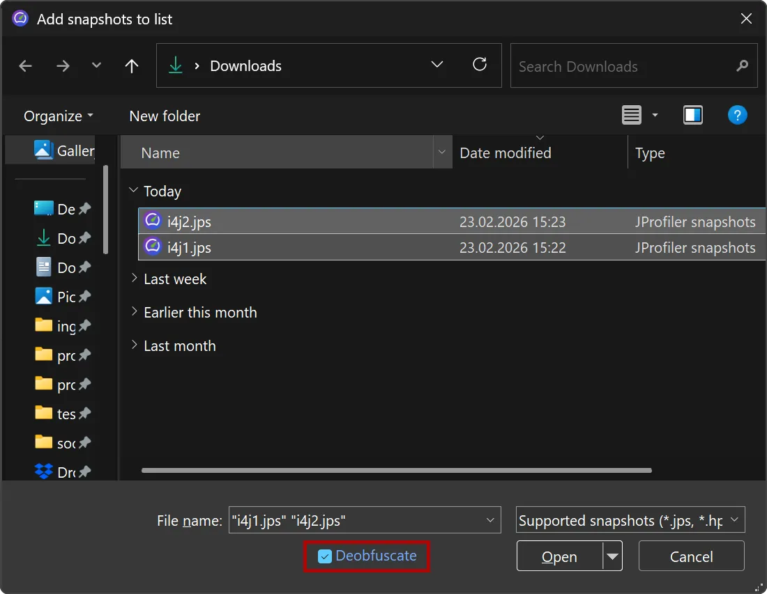
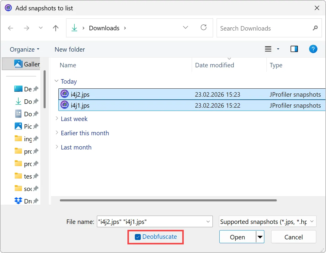
Similar to the existing deobfuscation support when opening snapshots, the file chooser now includes a "Deobfuscate" check box when
adding snapshots to the comparison window.
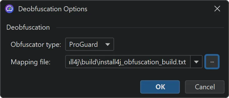
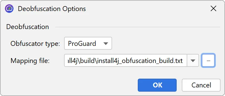
When selected, a dialog with a drop-down for supported obfuscators and a field for the mapping file path appears.
If different snapshot files have different mapping files, you can add the snapshots individually.
Once the mapping file is applied, all comparisons in JProfiler now show the original class and method names.
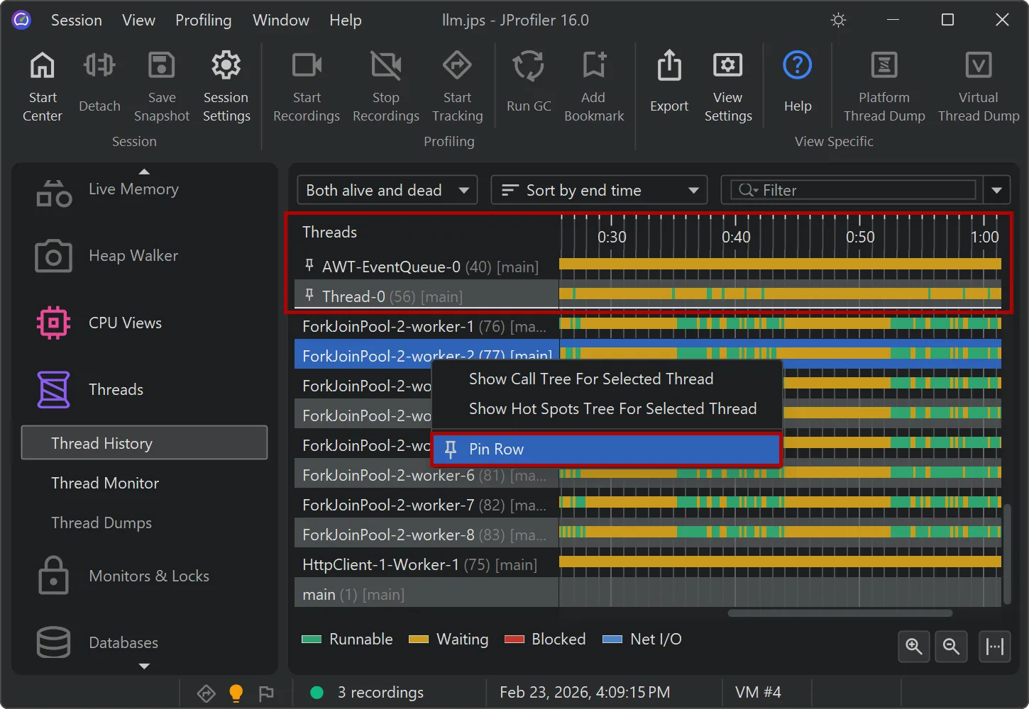
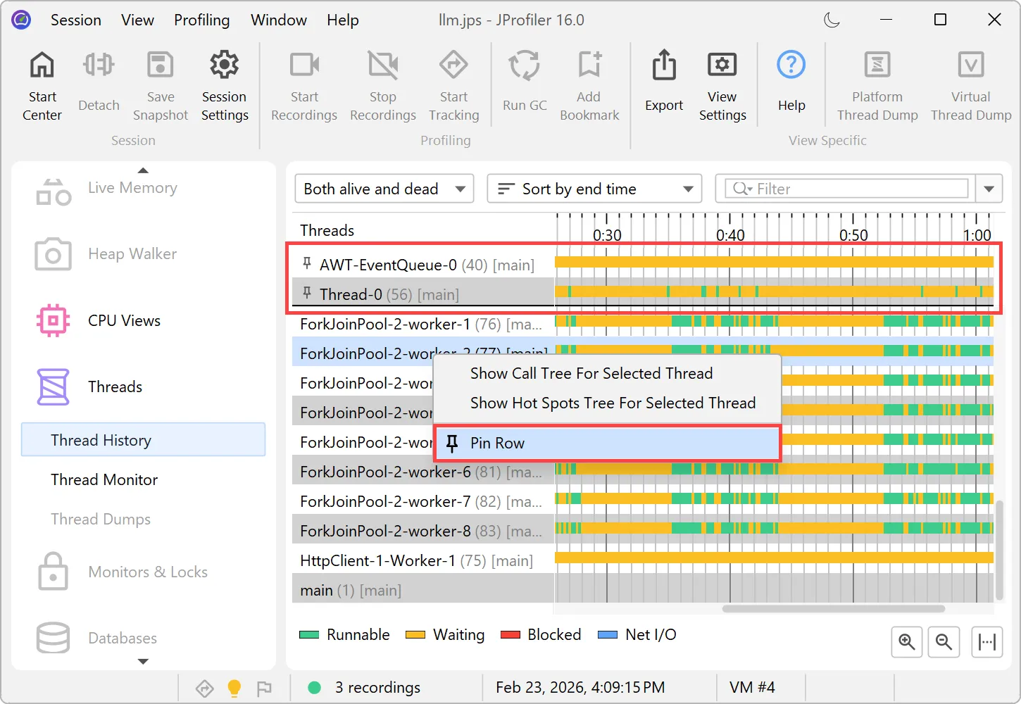
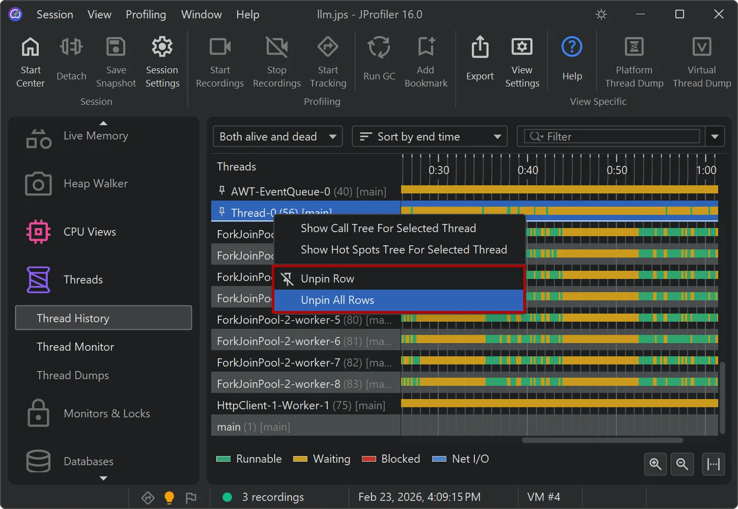
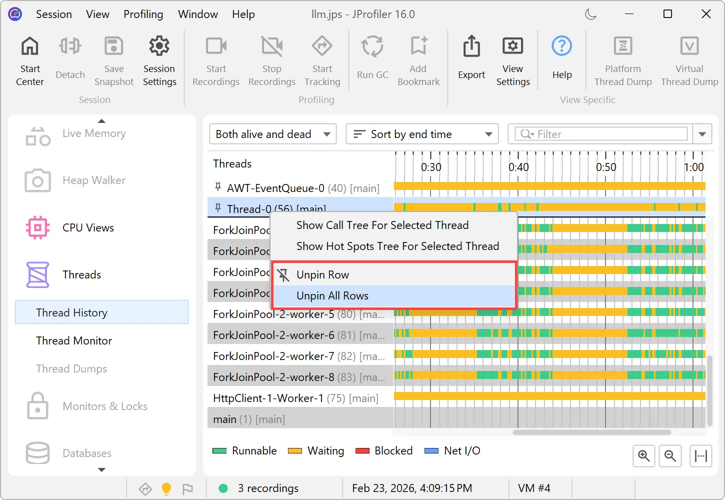
Timeline views now support row pinning.
In the threads history view and in all the probe timeline views, you can pin selected rows via the context menu. These are shown
in a separate area at the top where you can use drag and drop to change their order.
You can unpin pinned rows individually or all at once.
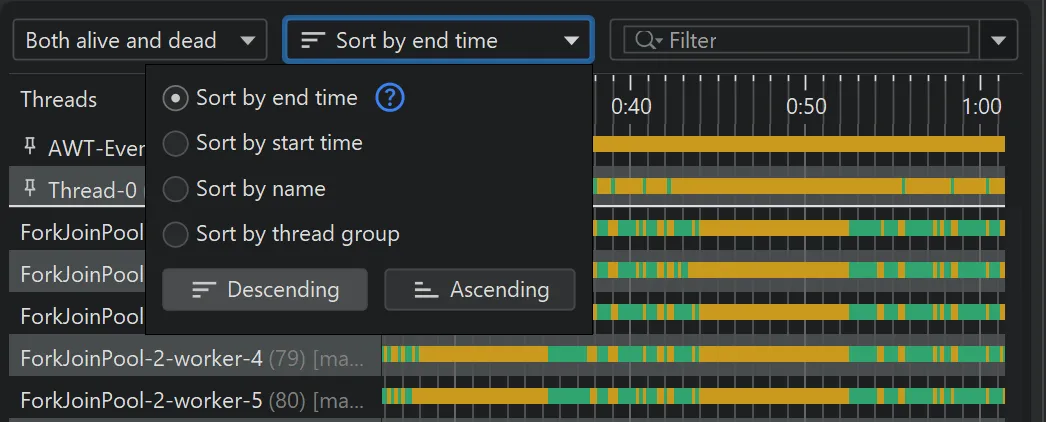
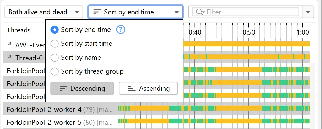
JProfiler 16 also introduces a sorting drop-down that offers ascending and descending sort directions and a new default sort mode
where active long-lived rows are shown first, followed by recently closed rows.
JProfiler 16 adds full support for profiling Java 26.
This version is essential if you are profiling virtual threads or if you are using the new built-in HTTP/3 support in the JDK HTTP client.
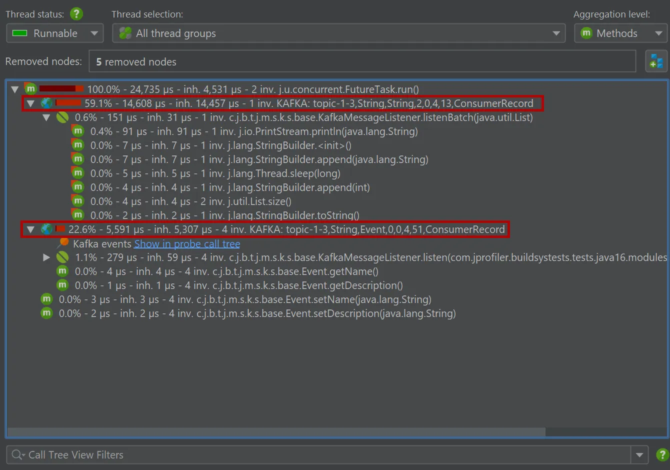
Probes for Apache Kafka were added. The probes measure various types of data that help you to identify
bottlenecks, optimize configurations, and maintain the health of your data streaming infrastructure.
To handle both client and server separately, there are separate probes for Kafka consumers and Kafka producers.
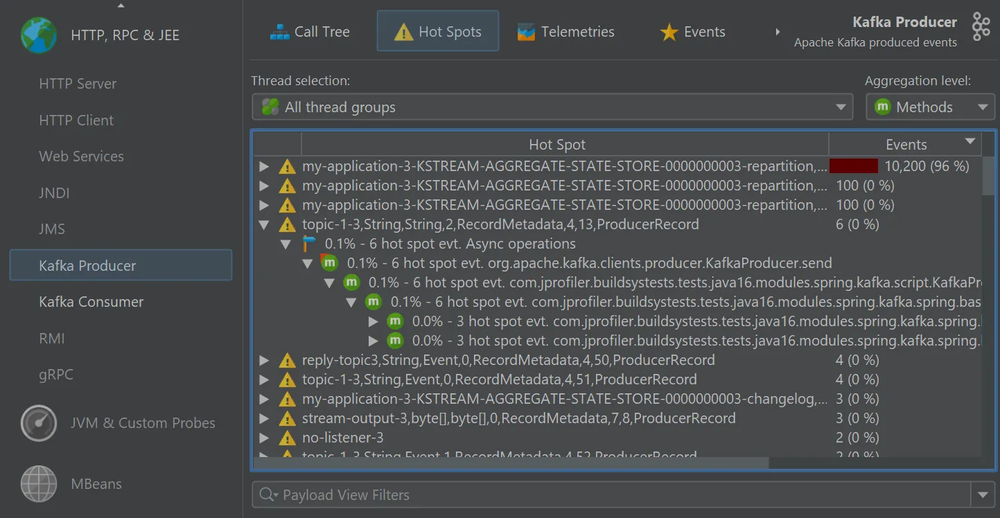
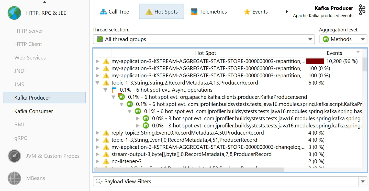
The "Kafka producer" probe analyzes the events that you publish.
A starting point for handling many kinds of problems is the "Hot spots" view where you can open hot spot nodes to see the back traces
into your code.
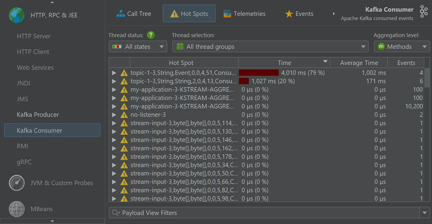
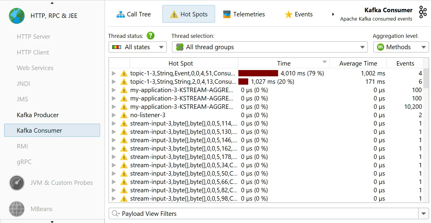
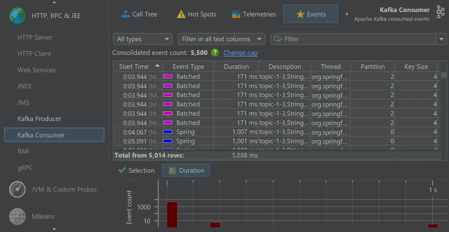
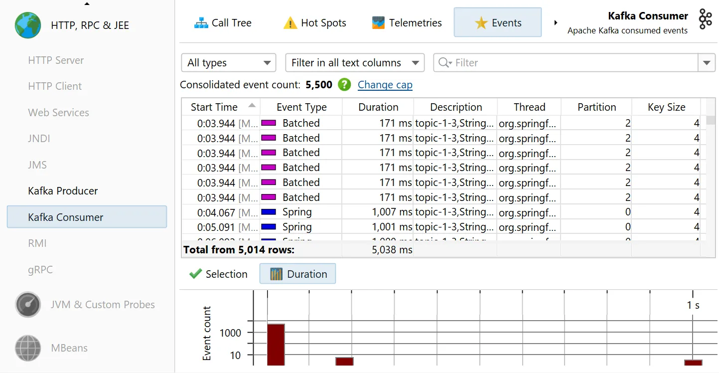
The "Kafka consumer" probe measures the events that you process. For Spring Kafka, event timings are recorded.
Single events can be analyzed in the "Events" view, where values for event type, thread name, partition, key and value size are also shown.
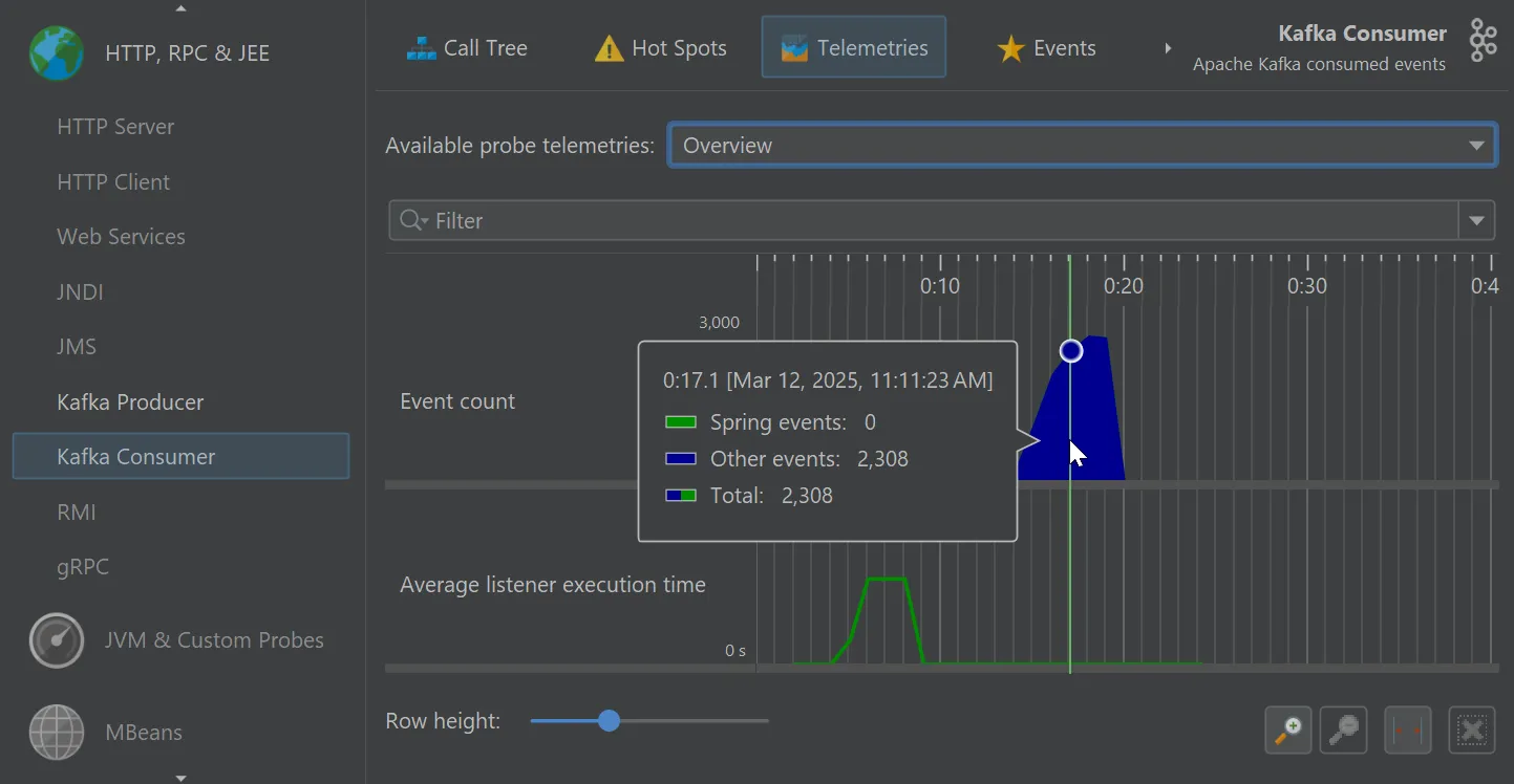
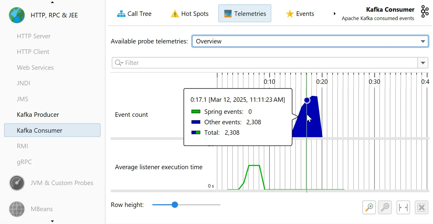
The Kafka probes contribute several telemetries, like "Event count" and "Average listener execution time" that can also be added
in the main "Telemetries" view section.
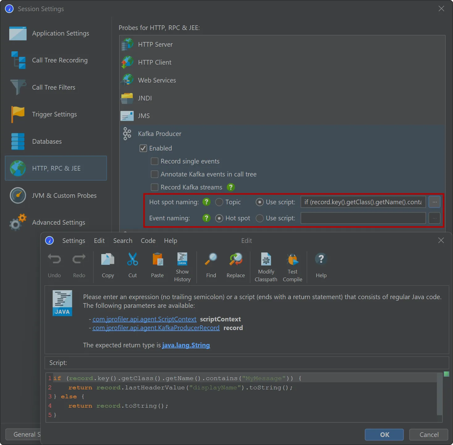
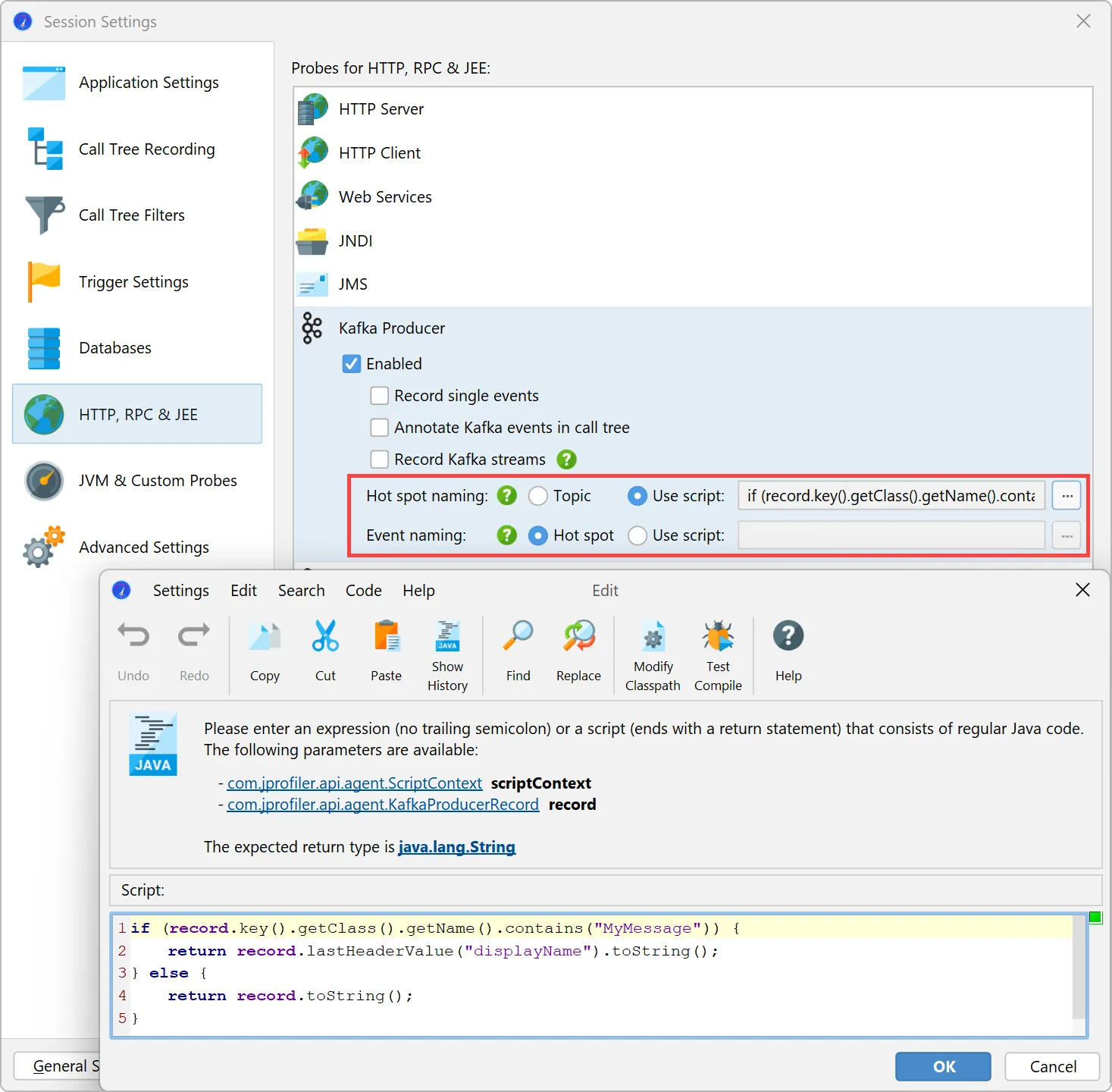
Both probes offer the same flexibility for naming hot spots and events. By default, hot spots are named with the message topic.
You can use a script to build the strings for the hot spots yourself using an API provided by JProfiler. Naming hot spots is important
because it determines the grouping in the hot spots view.
Optionally, you can use a different script for the naming of single events in the "Events" view. This will not affect hot spot grouping
and is a way to provide more detail for debugging.
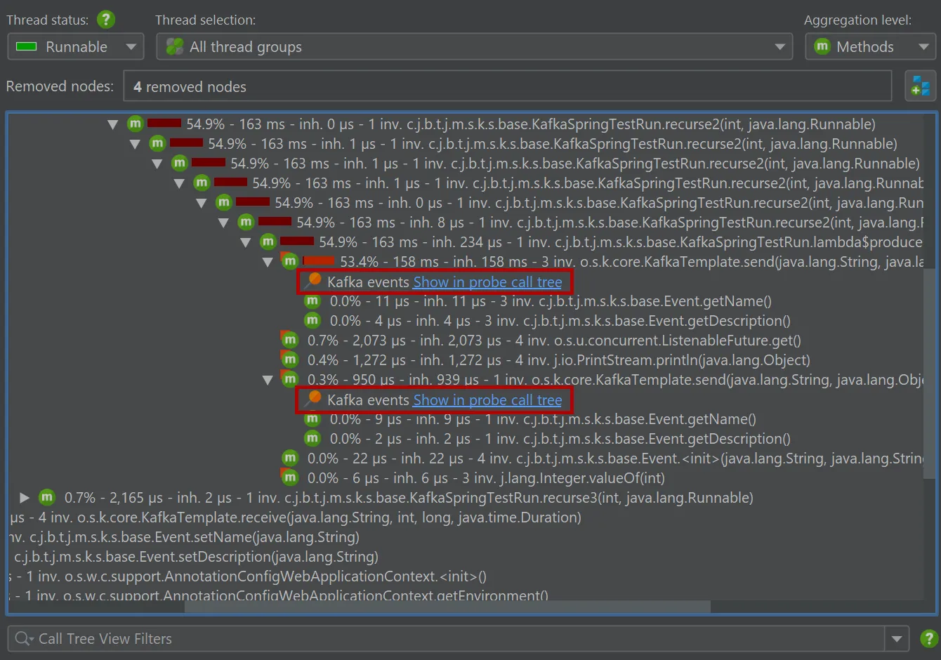
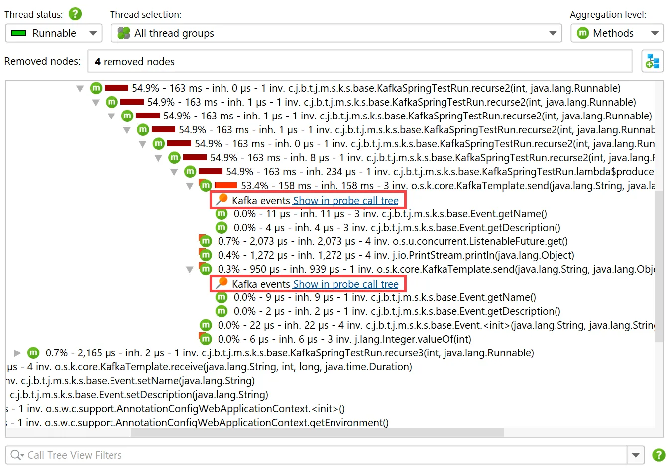
Recording events from either probe adds data in the regular call tree views in the "CPU views section". For the "Kafka producer" probe,
hyperlinks are inserted into the call tree for revealing the associated call stack in the call tree view of the probe.
The Kafka consumer probe splits the call tree for Spring event listeners, so you can see the subtree for different types of messages
separately. The grouping is done with the configured "hot spots" naming.
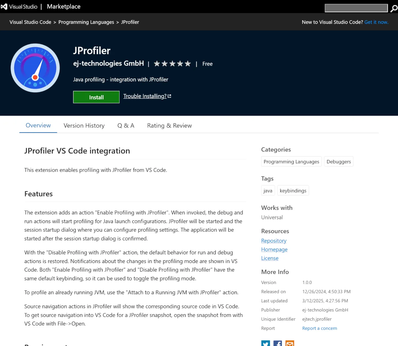
An IDE integration for Visual Studio Code has been added. It is available in the
Visual Studio Marketplace and works together with a
local installation of JProfiler.
If the VS Code plugin cannot find the JProfiler installation automatically, it will ask you to locate it the first time you start a profiling
session.
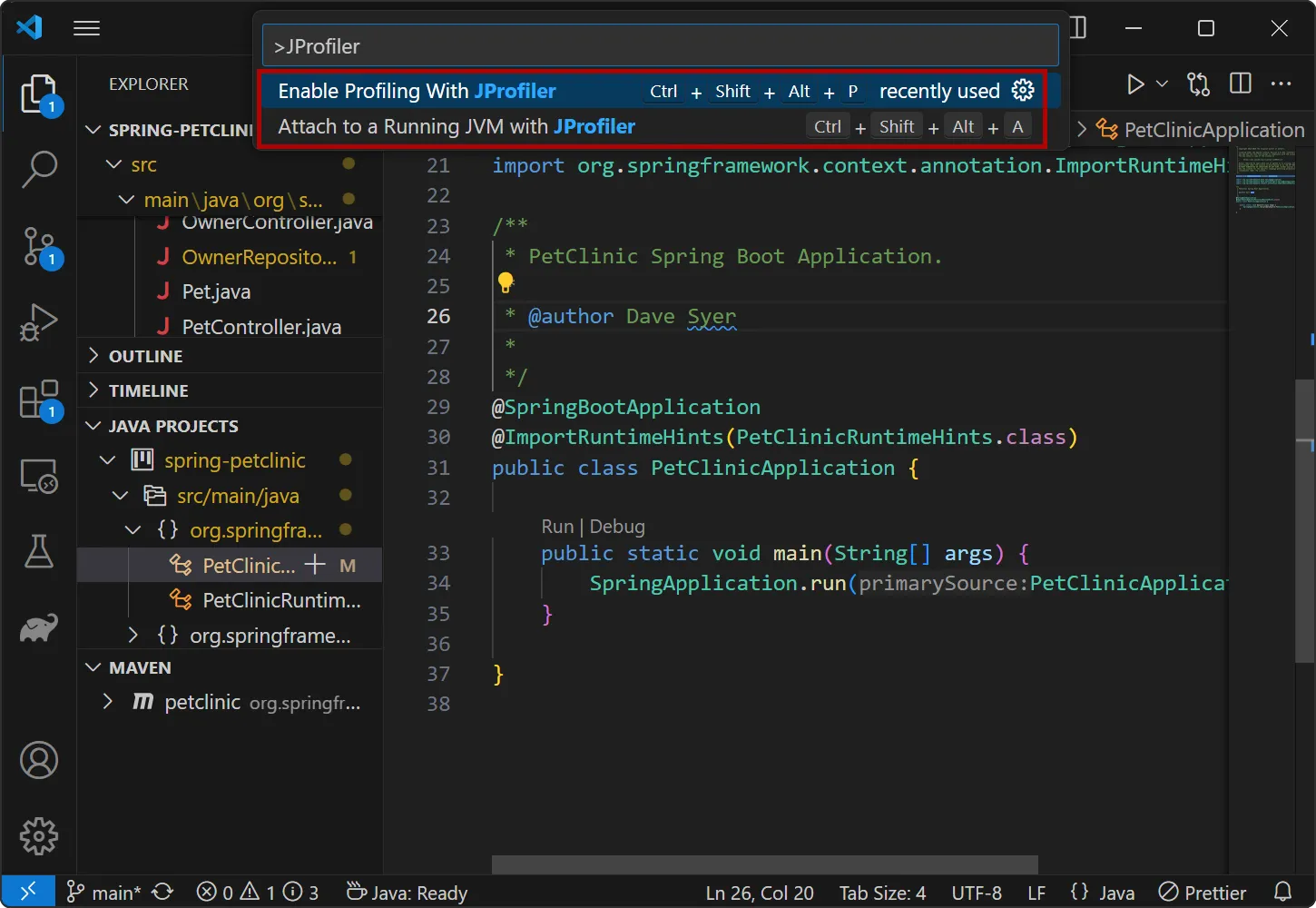
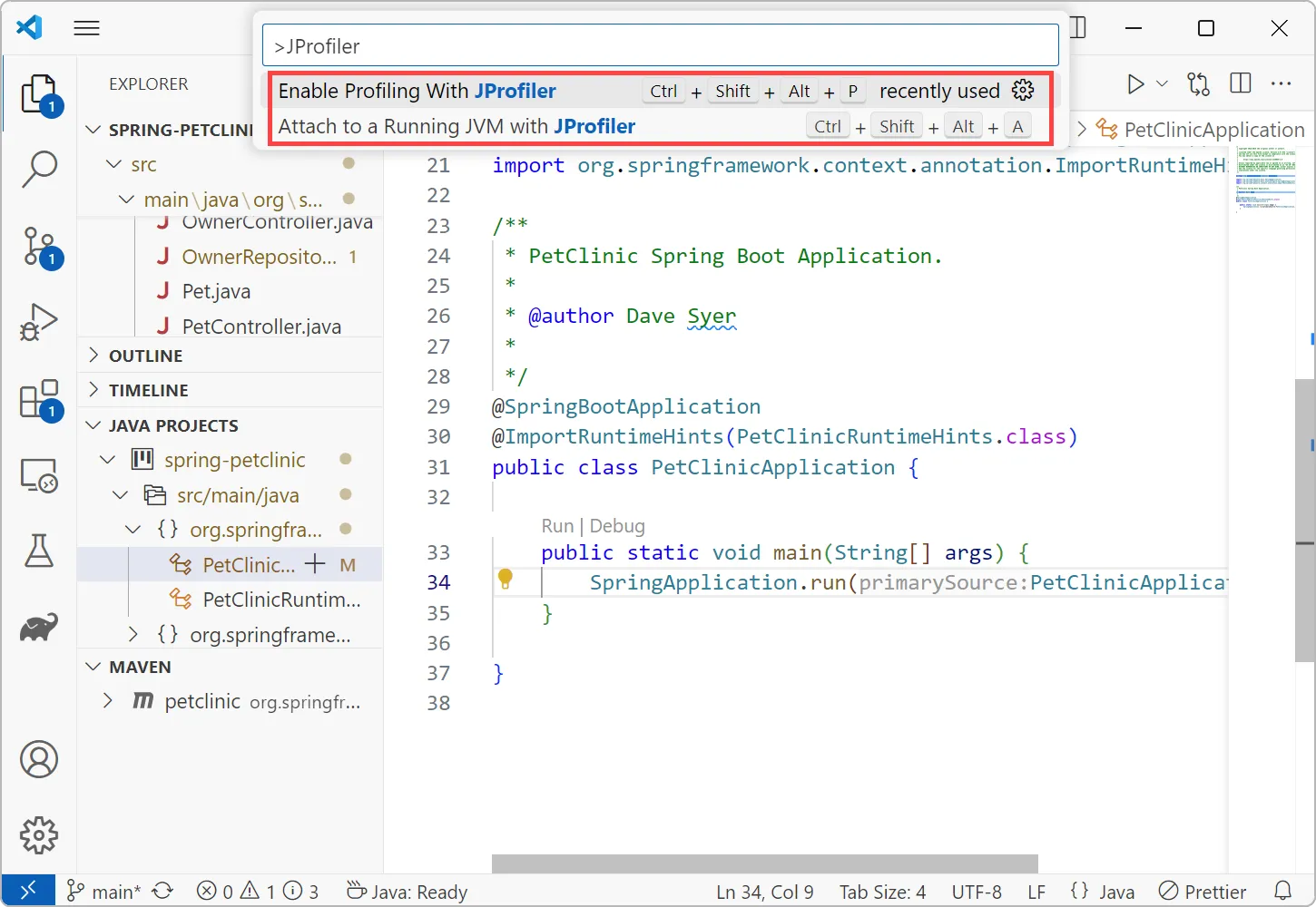
The extension adds two actions: With "Enable Profiling with JProfiler" you toggle the profiling mode, so that all debug and run actions
will start profiling for Java launch configurations. With "Attach to a running JVM with JProfiler" you can use the attach mode feature for
local or remote JVMs and get source code navigation into VS code.
Depending on the status of this pull request for the vscode-gradle
plugin, profiling Gradle tasks is also supported by the "Enable Profiling with JProfiler" action.
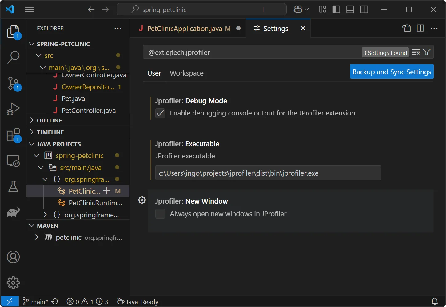
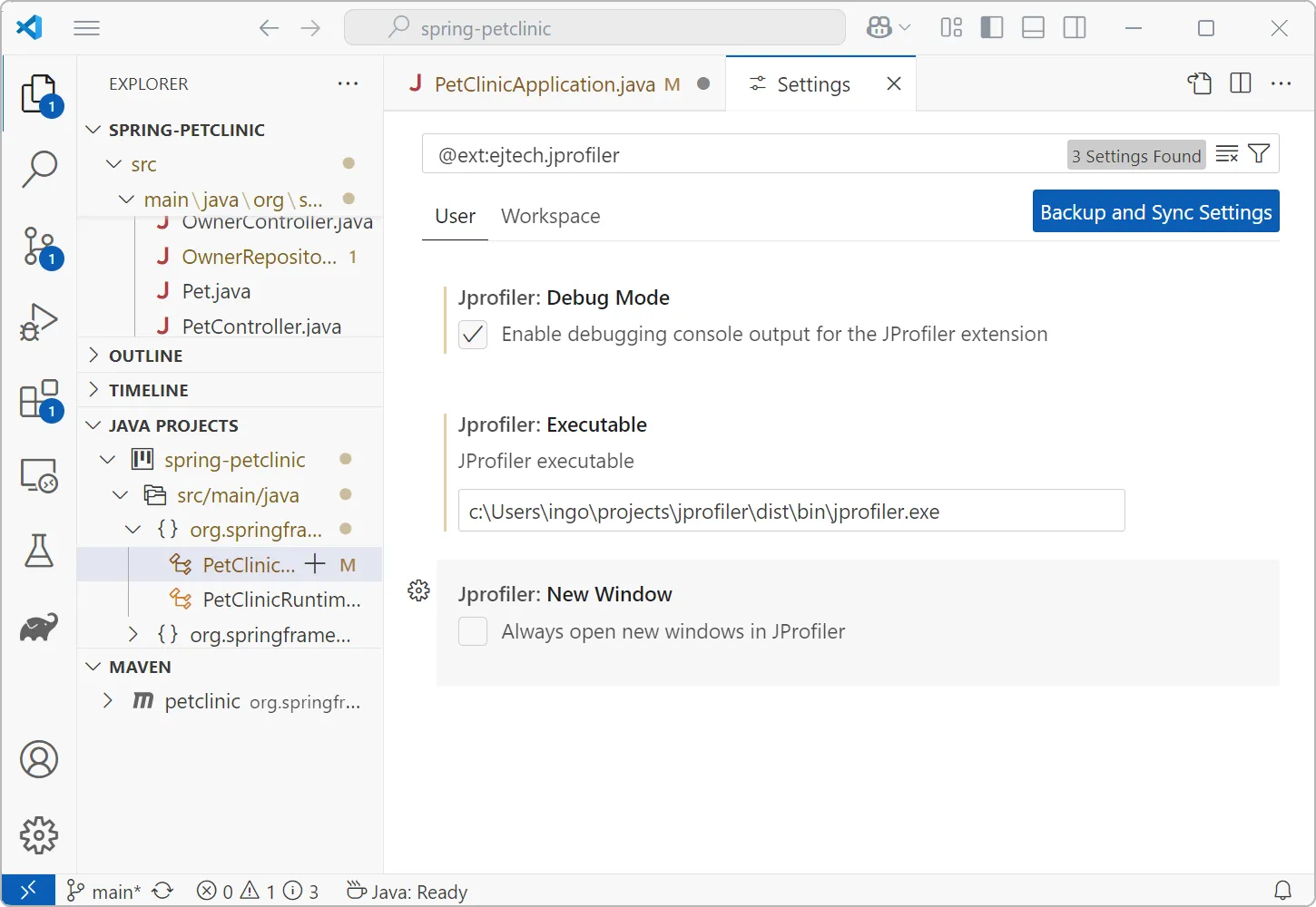
The JProfiler plugin only has a few settings, notably for the location of the JProfiler executable and a setting whether to open new windows
for new profiling sessions.
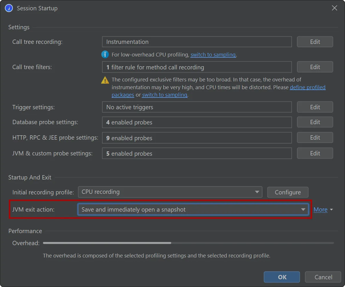
All other profiling settings are handled by JProfiler and stored on a per-project basis. When you start a profiling session, the
session startup dialog gives you a chance to view and modify all settings in one place.
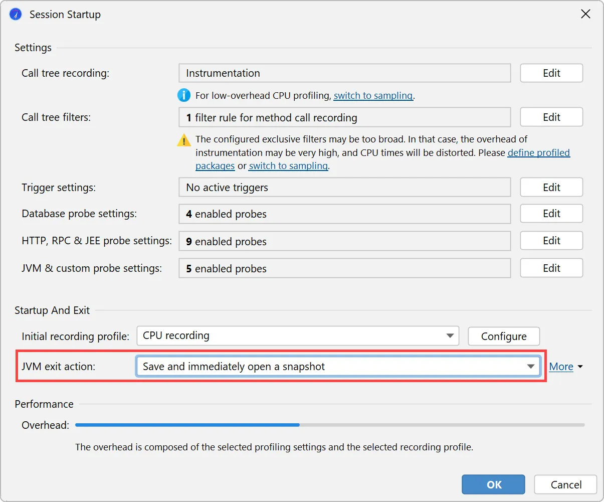
When profiling unit tests, JProfiler will automatically suggest saving and immediately opening a snapshot when the JVM exits.
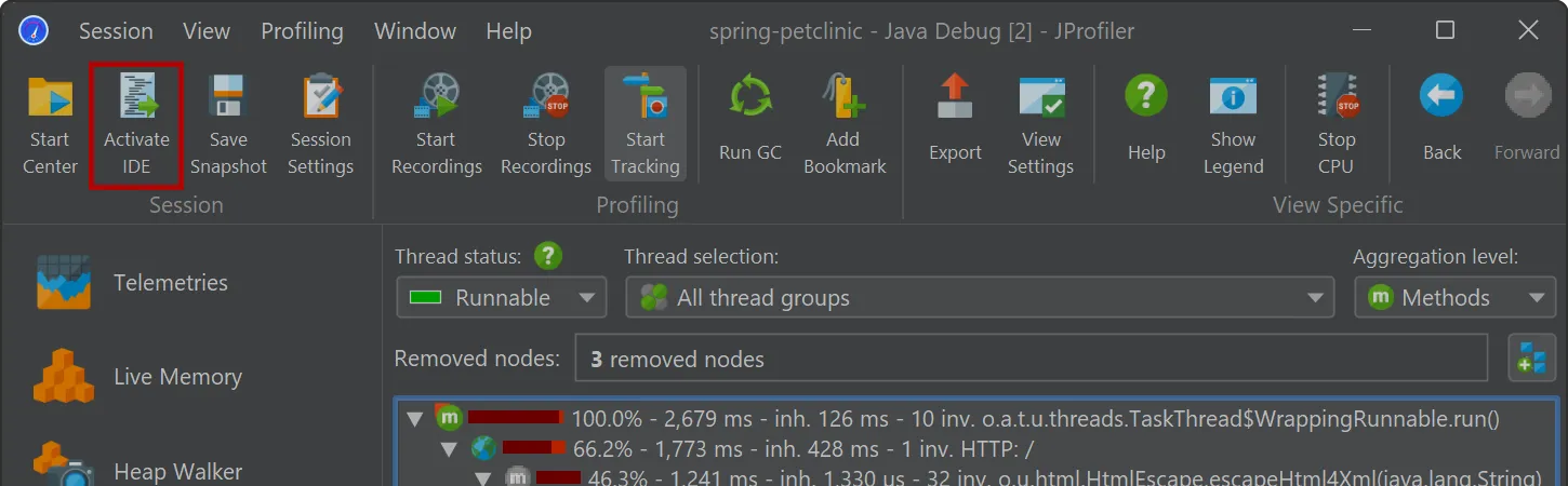
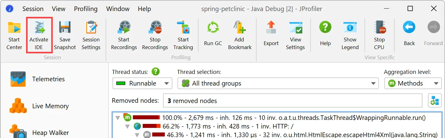
Switching to VS code when working with the JProfiler UI is seamlessly possible with the "Activate IDE" action (F11).
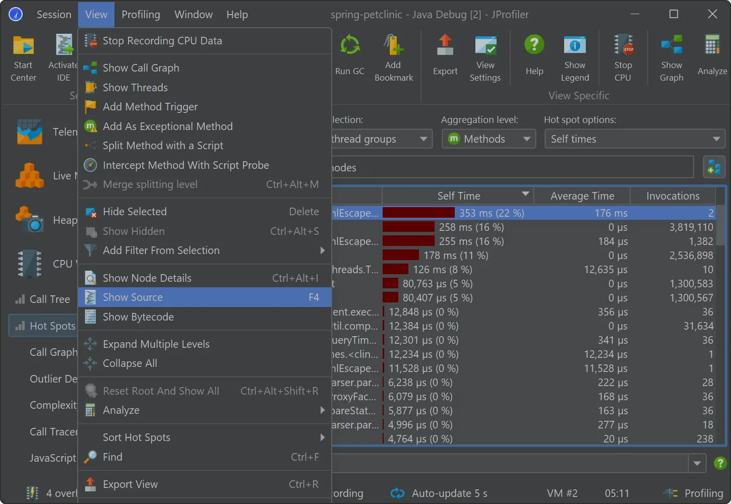
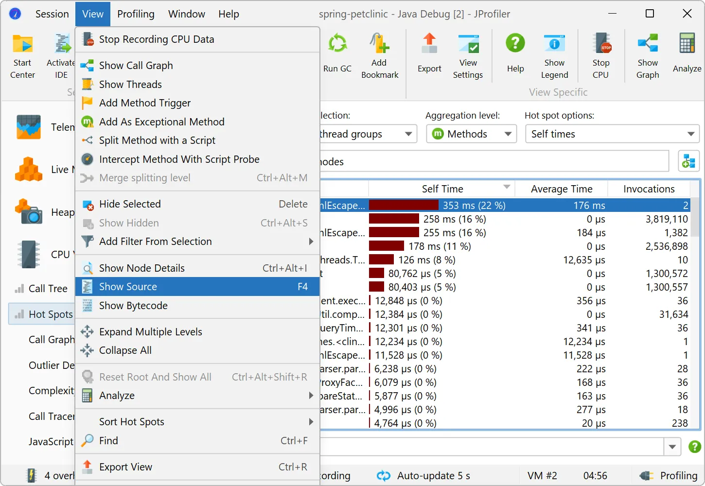
To show the source code of a selected class or method, use the "Show source" action that is visible everywhere in JProfiler. The VS
Code UI will be brought to the front, and the associated source code will be shown.
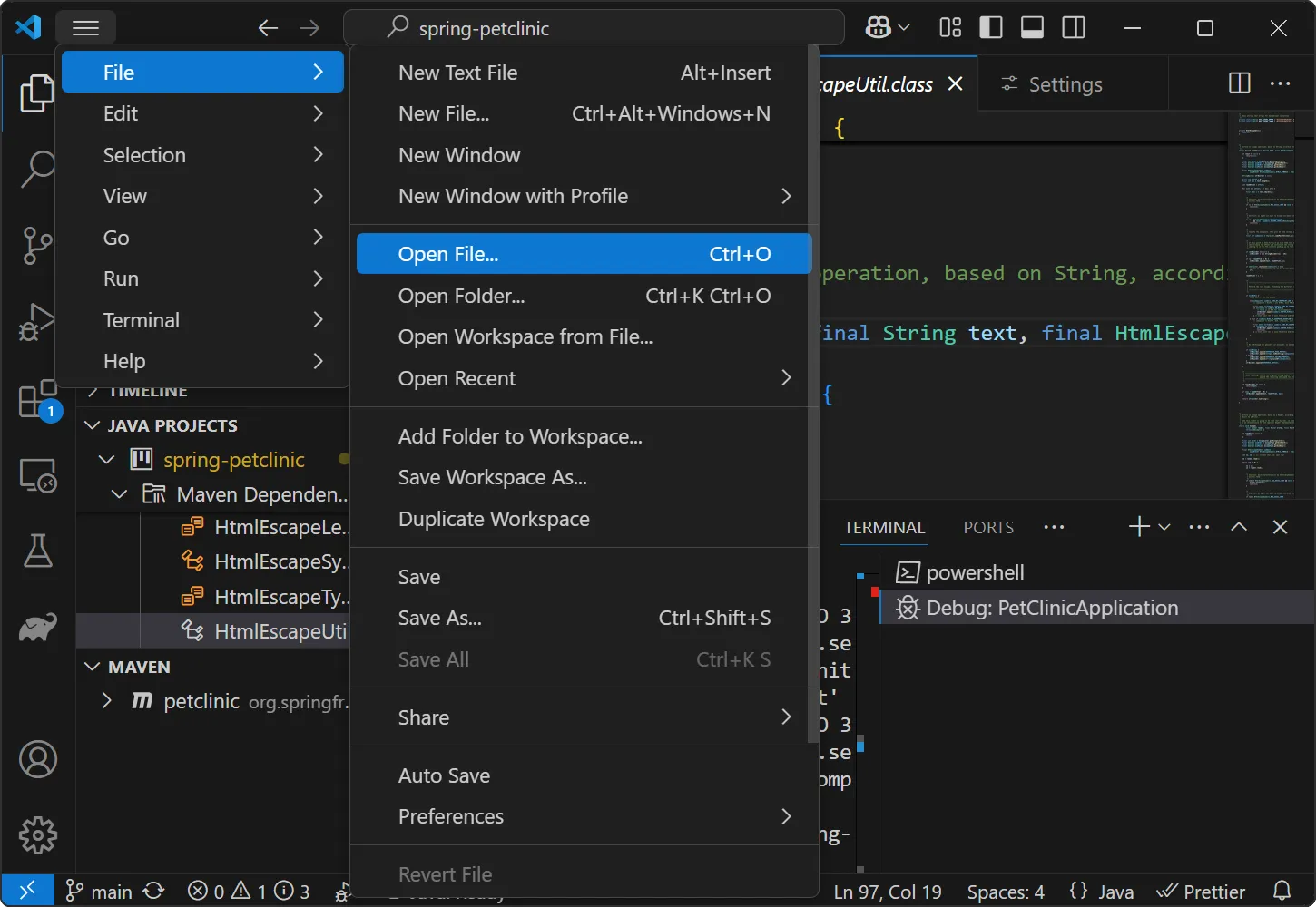
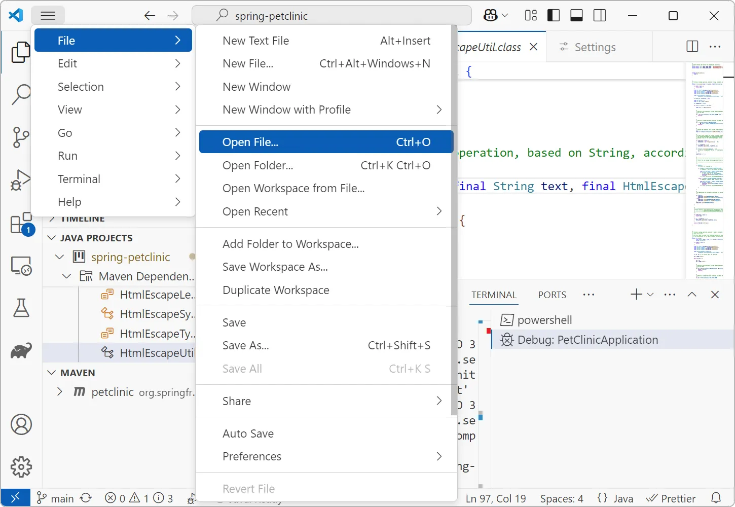
Another useful feature provided by the JProfiler VS Code plugin is that you can open JProfiler, HPROF and PHD snapshots from inside
VS Code to get source code navigation from the JProfiler UI into VS Code.
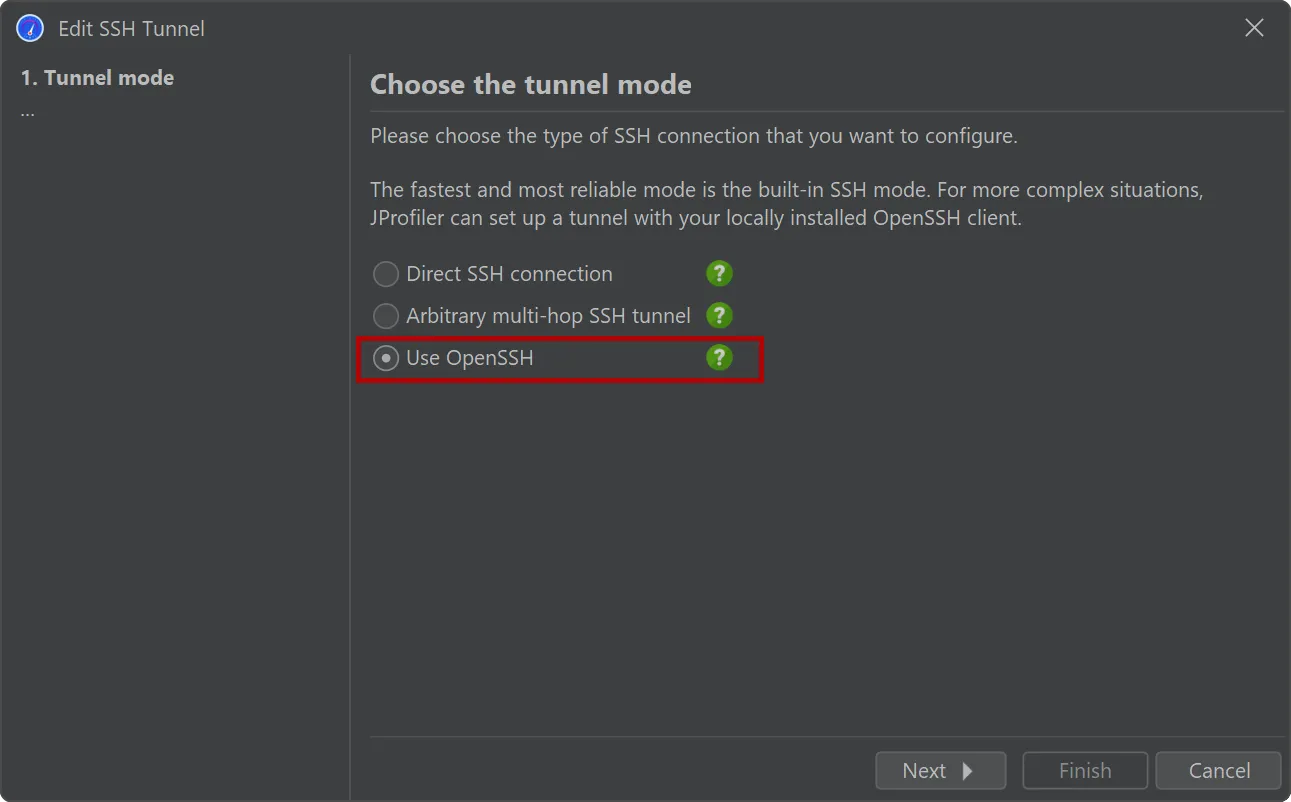
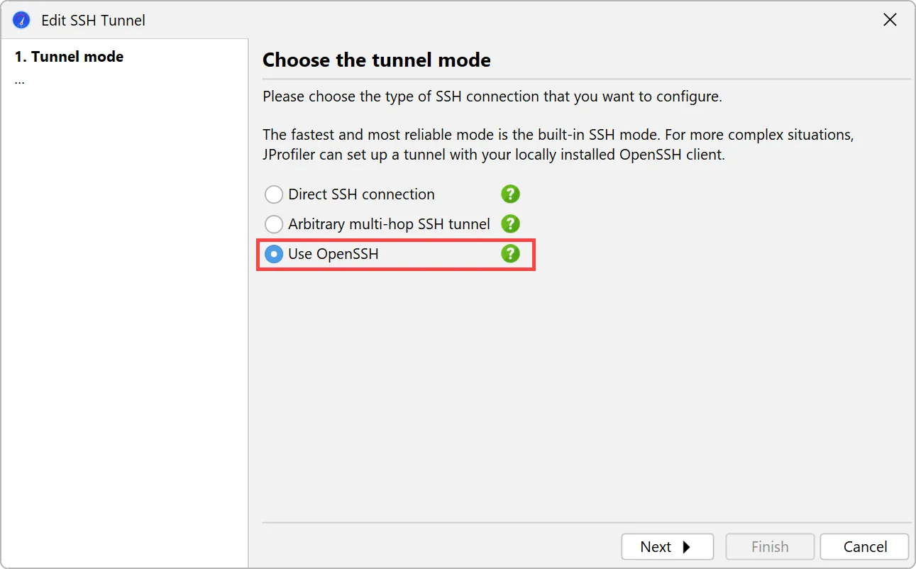
An alternative SSH mode via OpenSSH has been added. This is important for being able to profile JVMs on all types of remote
machines without any configuration.
JProfiler ships with a built-in SSH client for SSH connections that supports password and public key authentication. To support
other authentication types and complex network topologies, a new SSH tunnel type was added, that uses your local OpenSSH installation.
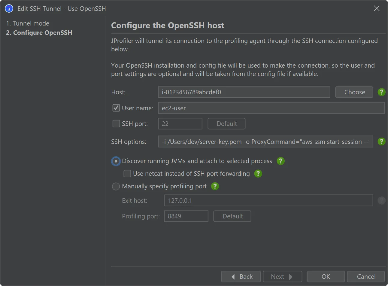
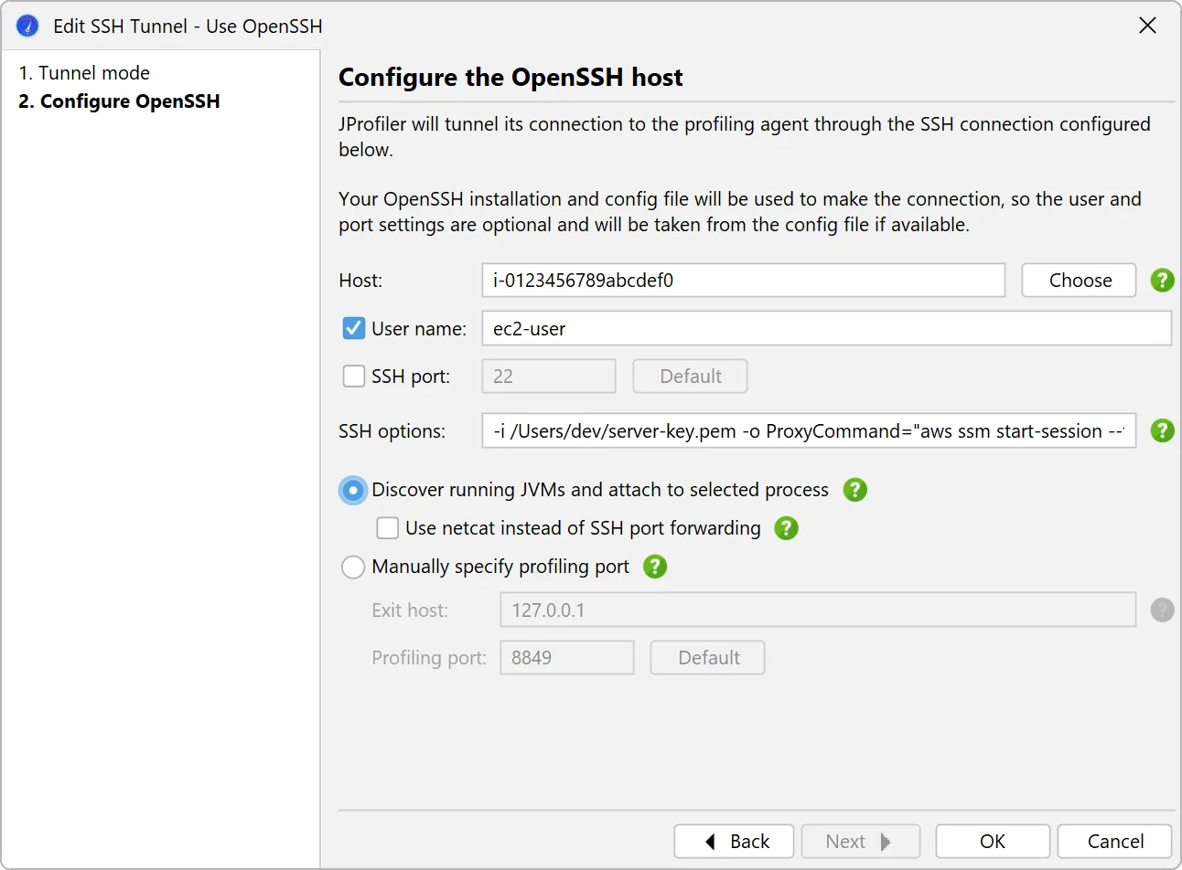
For example, if you want to connect to an EC2 instance via AWS session manager, the built-in SSH client does not work because it cannot
tunnel through an arbitrary proxy. In the
AWS documentation,
you get a list of options that you can either add to the OpenSSH config file or directly on the command line, both of which work with the
new OpenSSH mode in JProfiler. This involves a ProxyCommand option that tunnels the connection through the aws
executable. In the screenshot below, the "SSH options" text field contains these arguments.
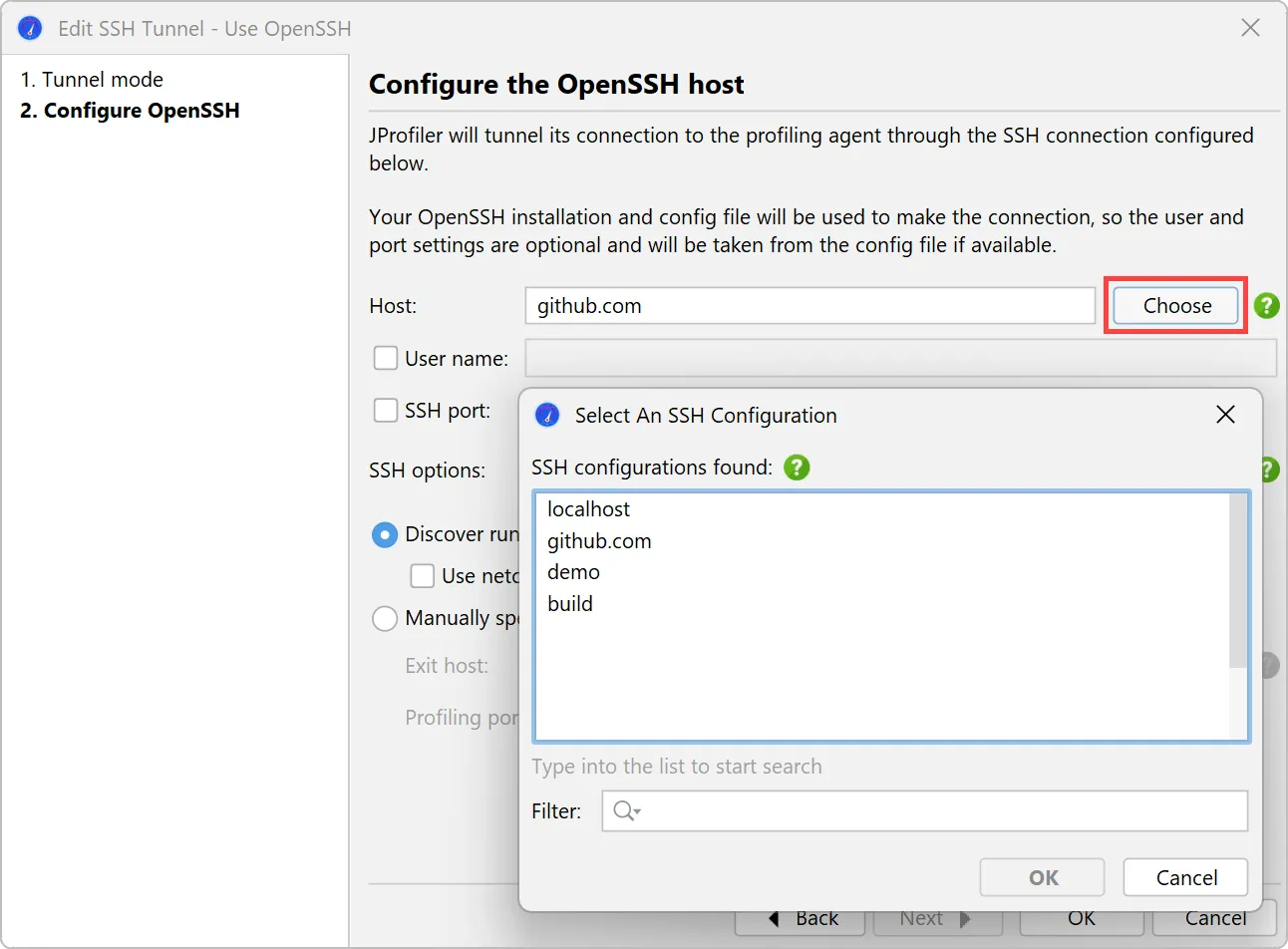
The only required input for the OpenSSH mode is the host name.
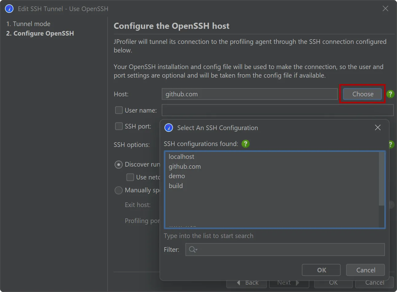
In the case where you use the OpenSSH config file to define your fully configured SSH servers, you can easily
select them with the "Choose" button next to the "Host" text field.
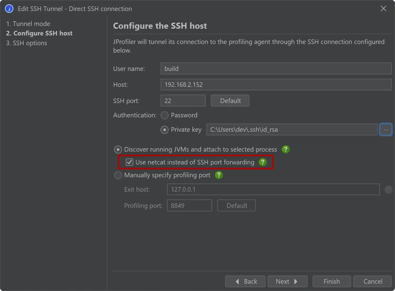
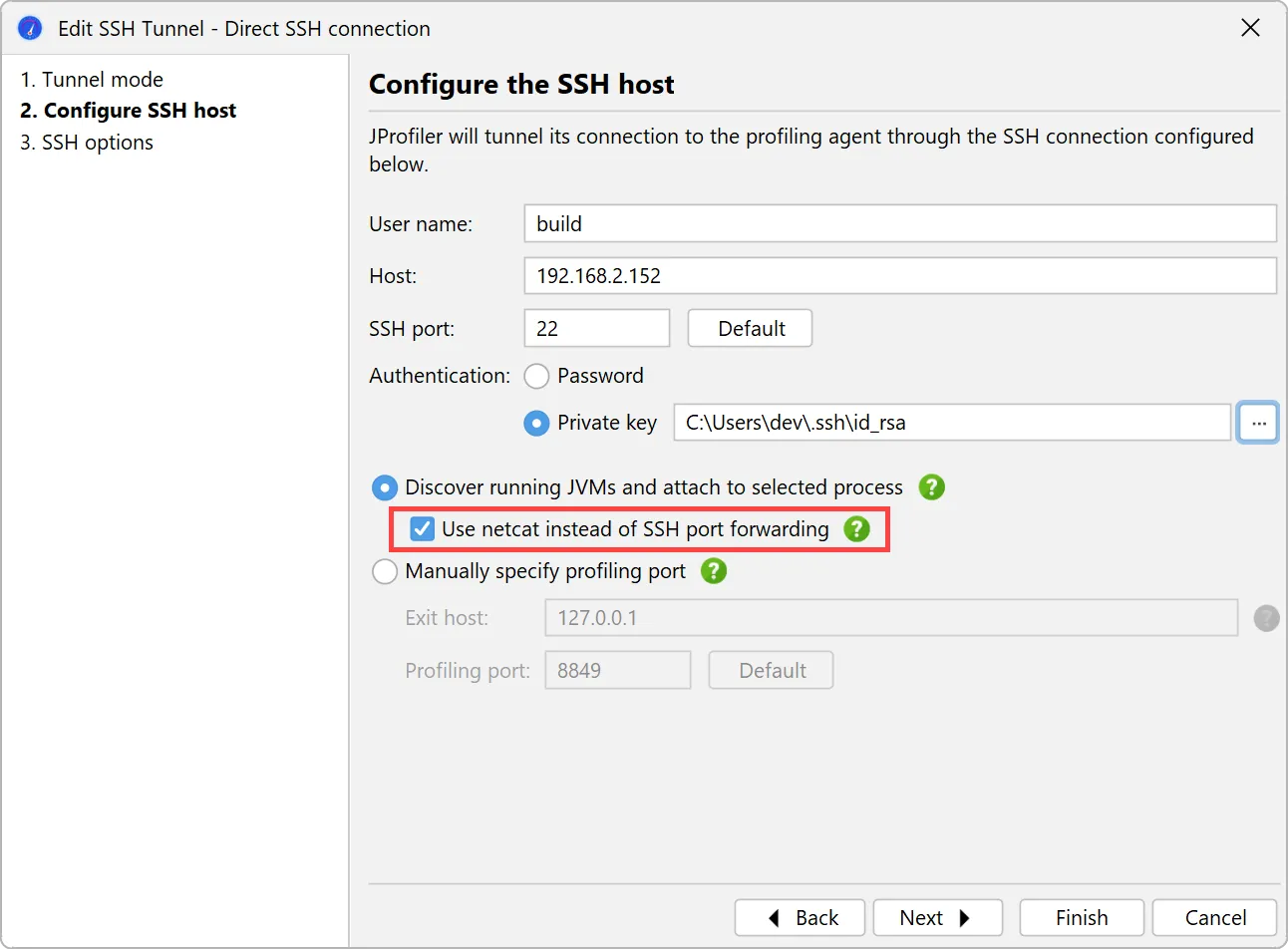
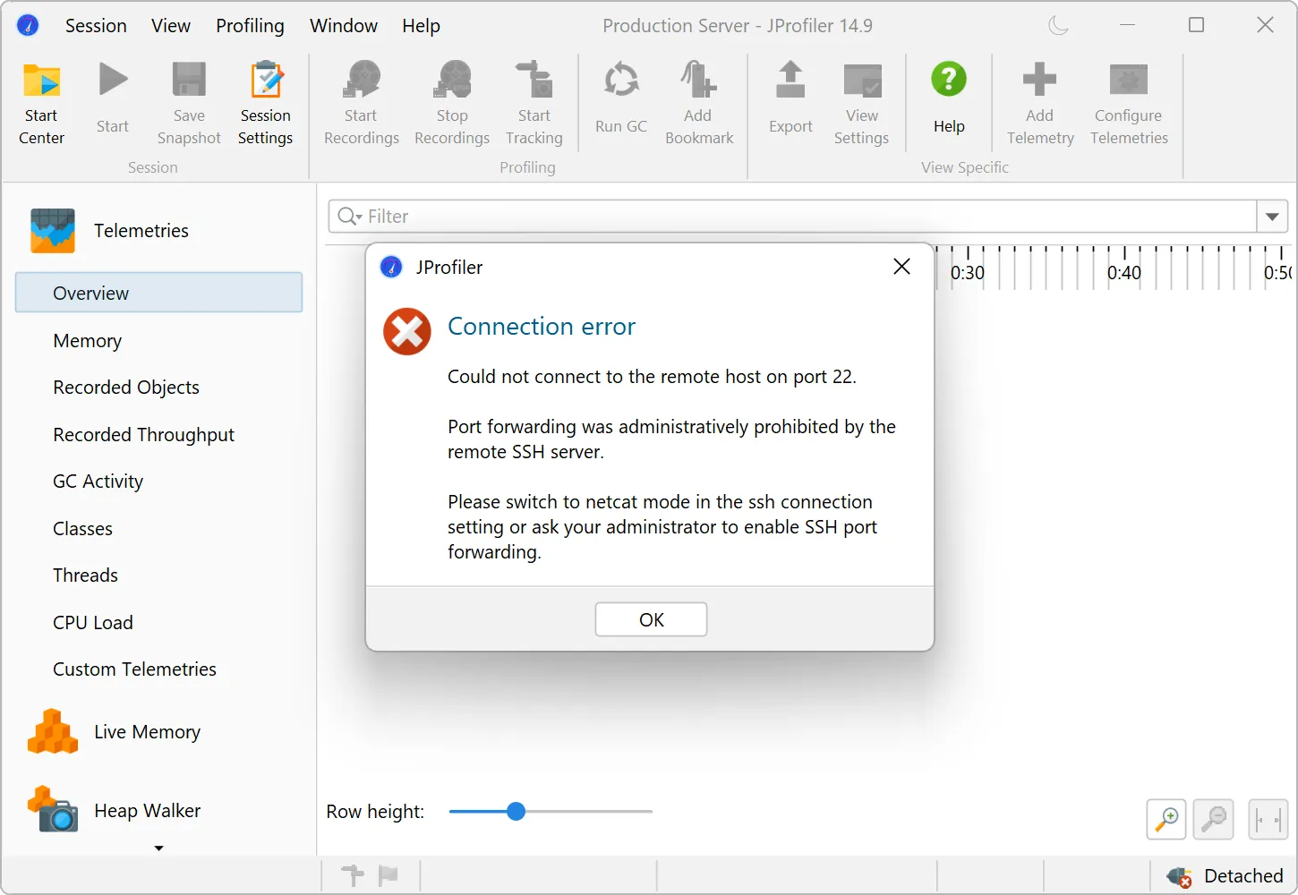
An alternative netcat SSH mode has been added for SSH hosts where port forwarding is disabled.
Many security-hardened production systems disable SSH port forwarding. In those cases, previous versions of JProfiler could not establish
an SSH tunnel through such machines. While SSH port forwarding is still the preferred option for SSH connections due to its stability and
better error reporting, JProfiler 15 adds a "netcat mode" that can optionally be enabled to fix this issue.
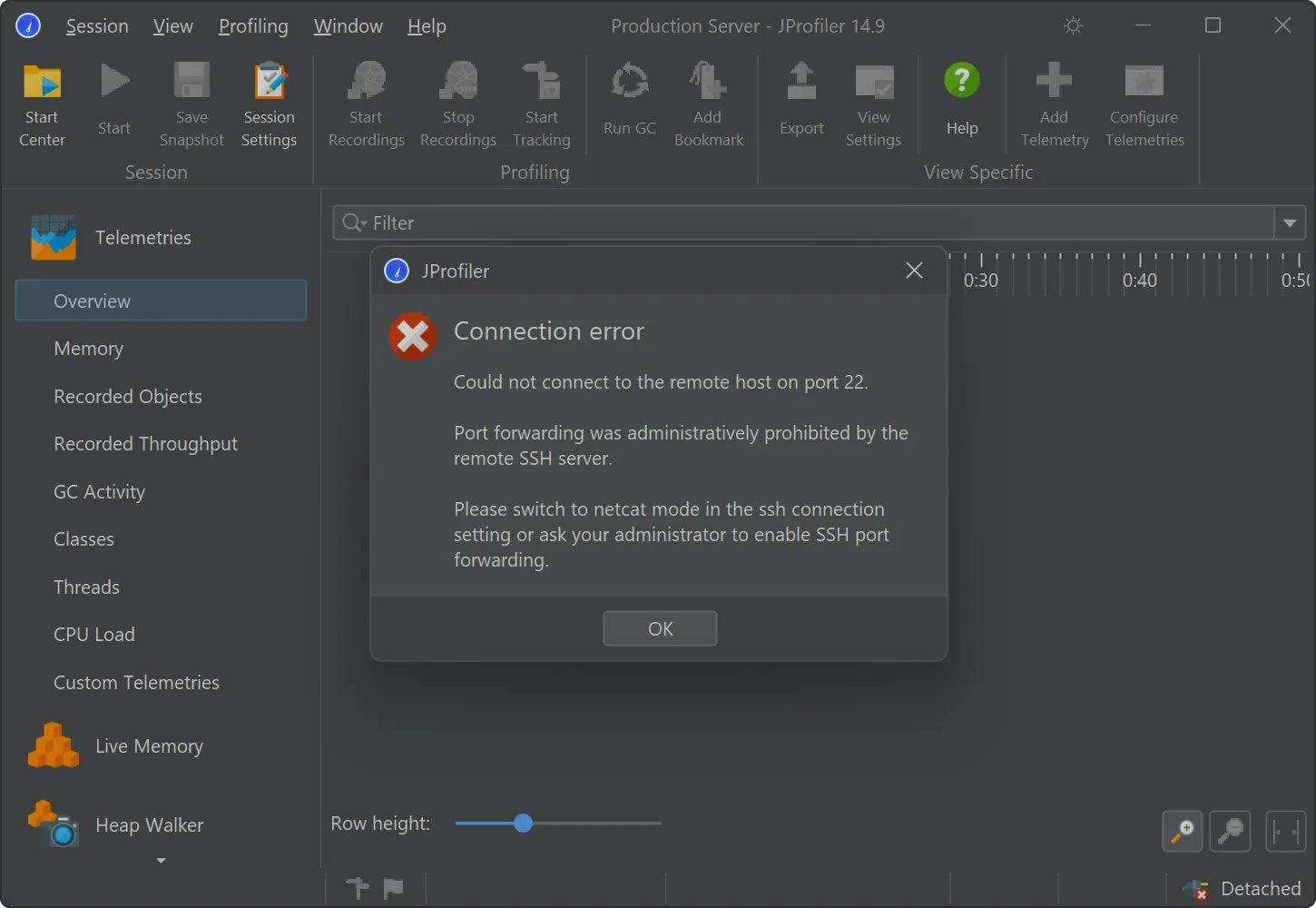
When a connection fails in such a way that disabled port forwarding may be to blame, JProfiler suggest switching to the netcat mode.
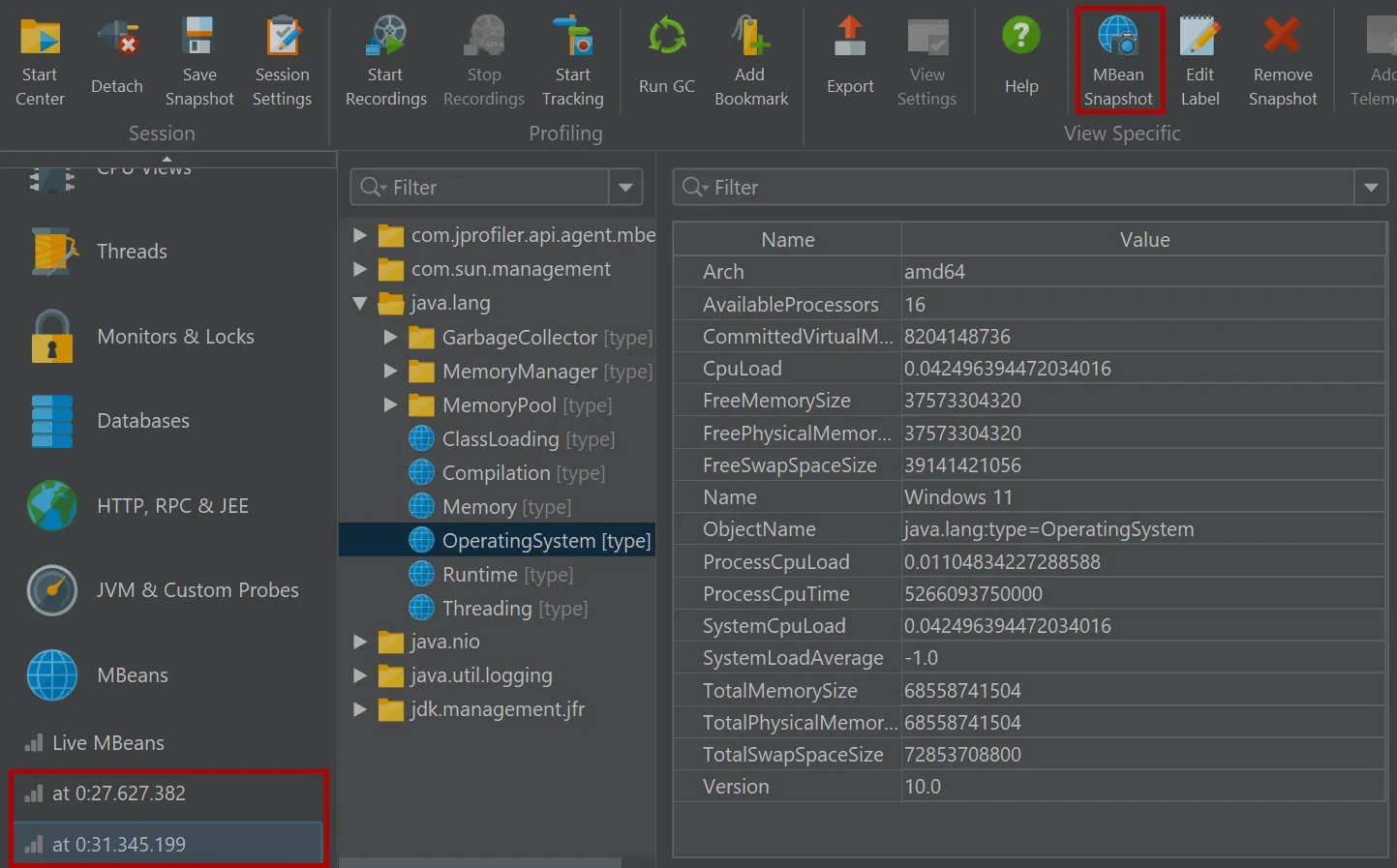
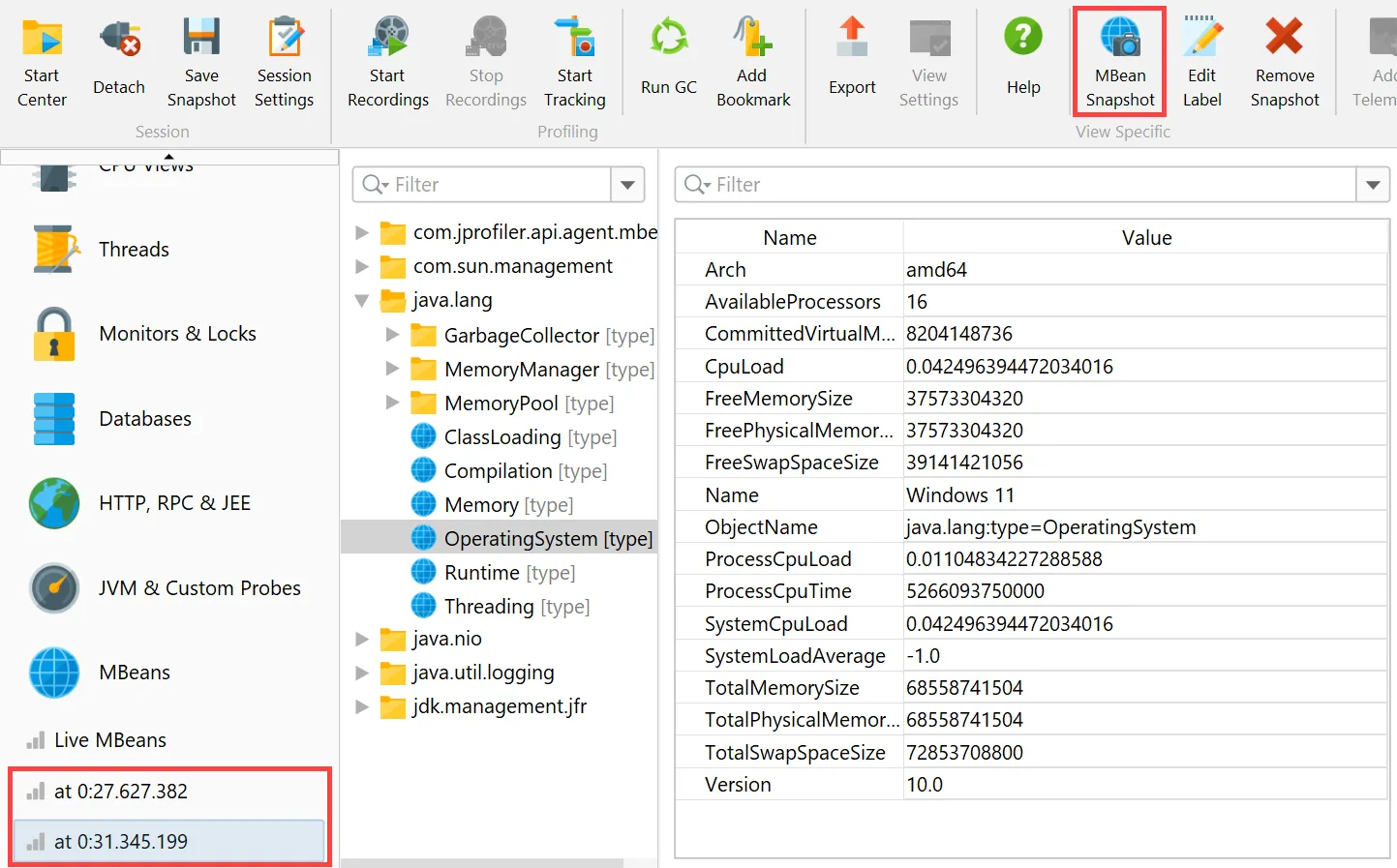
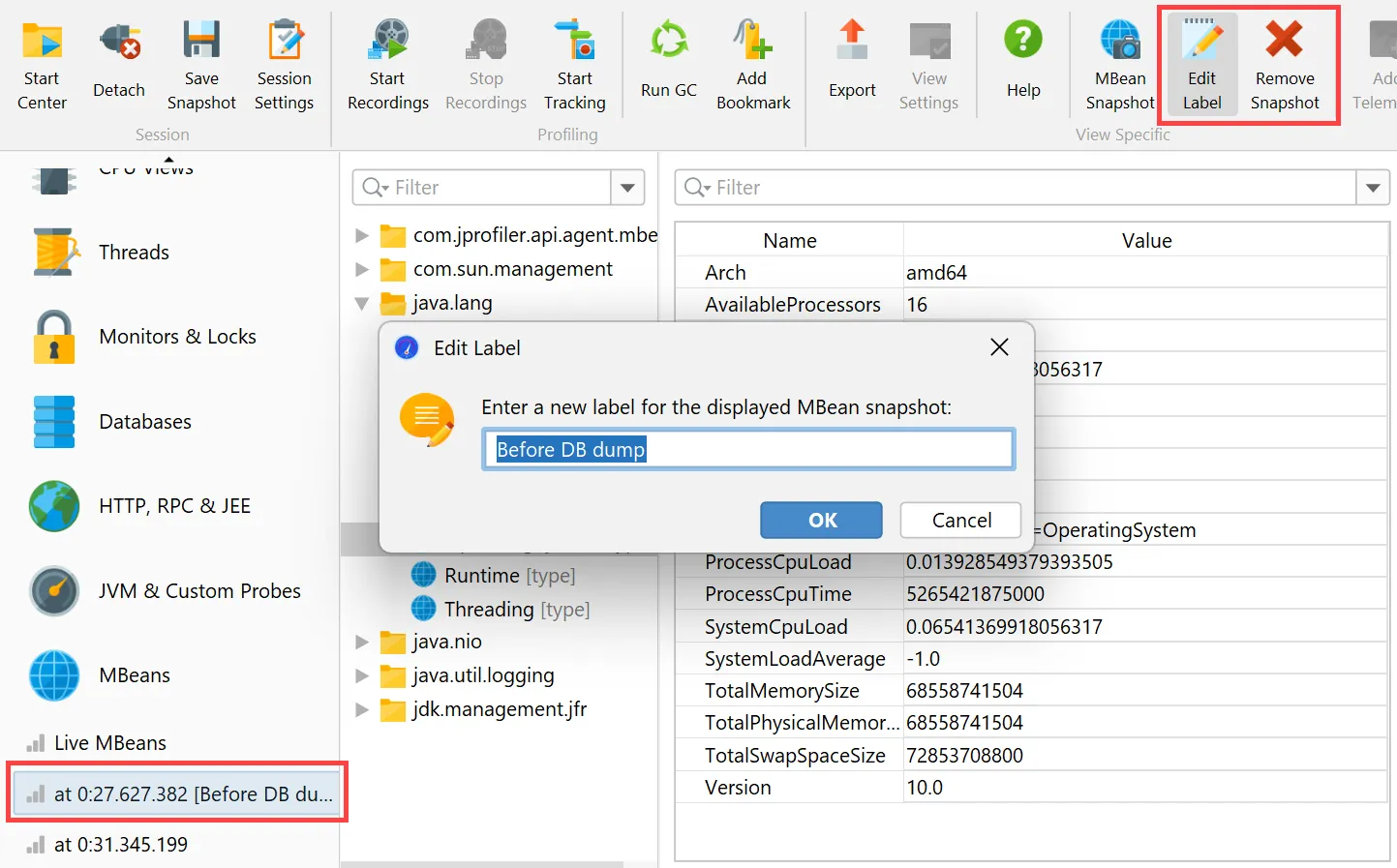
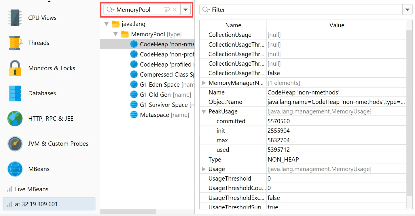
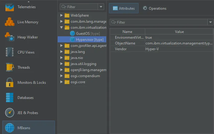
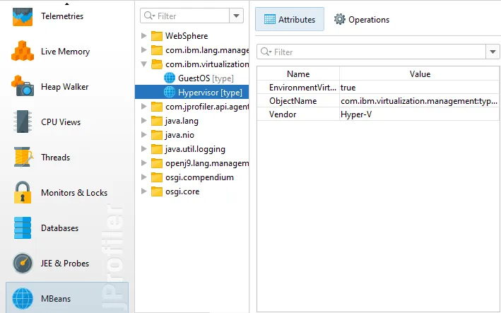
JProfiler can now take MBean snapshots. This is especially useful if you save JProfiler snapshots, either from the UI
or during offline profiling. MBean snapshots enable you to use the MBean browser when JProfiler is not attached to the live JVM.
In live mode, the "MBean snapshot" action in the toolbar creates a new snapshot that is then shown in the view selector. You can take
multiple snapshots and switch between them.
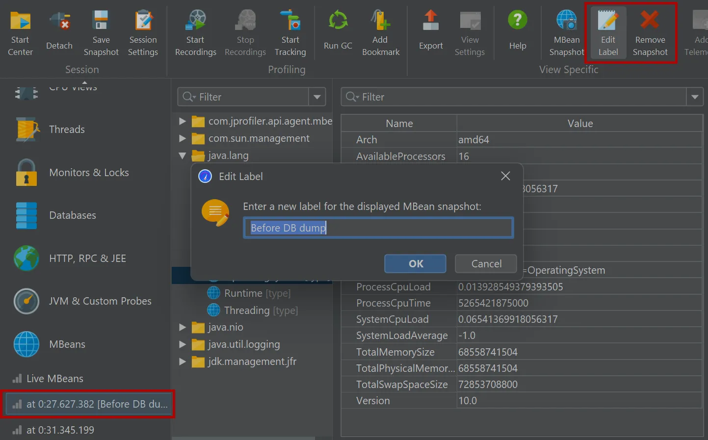
MBean snapshots can be assigned labels that are displayed in the view selector. Unwanted MBean snapshots can also be removed again.
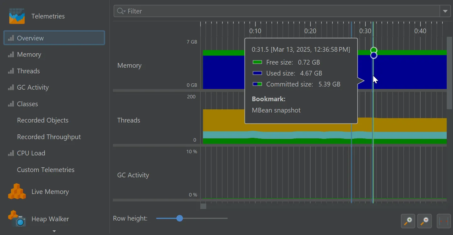
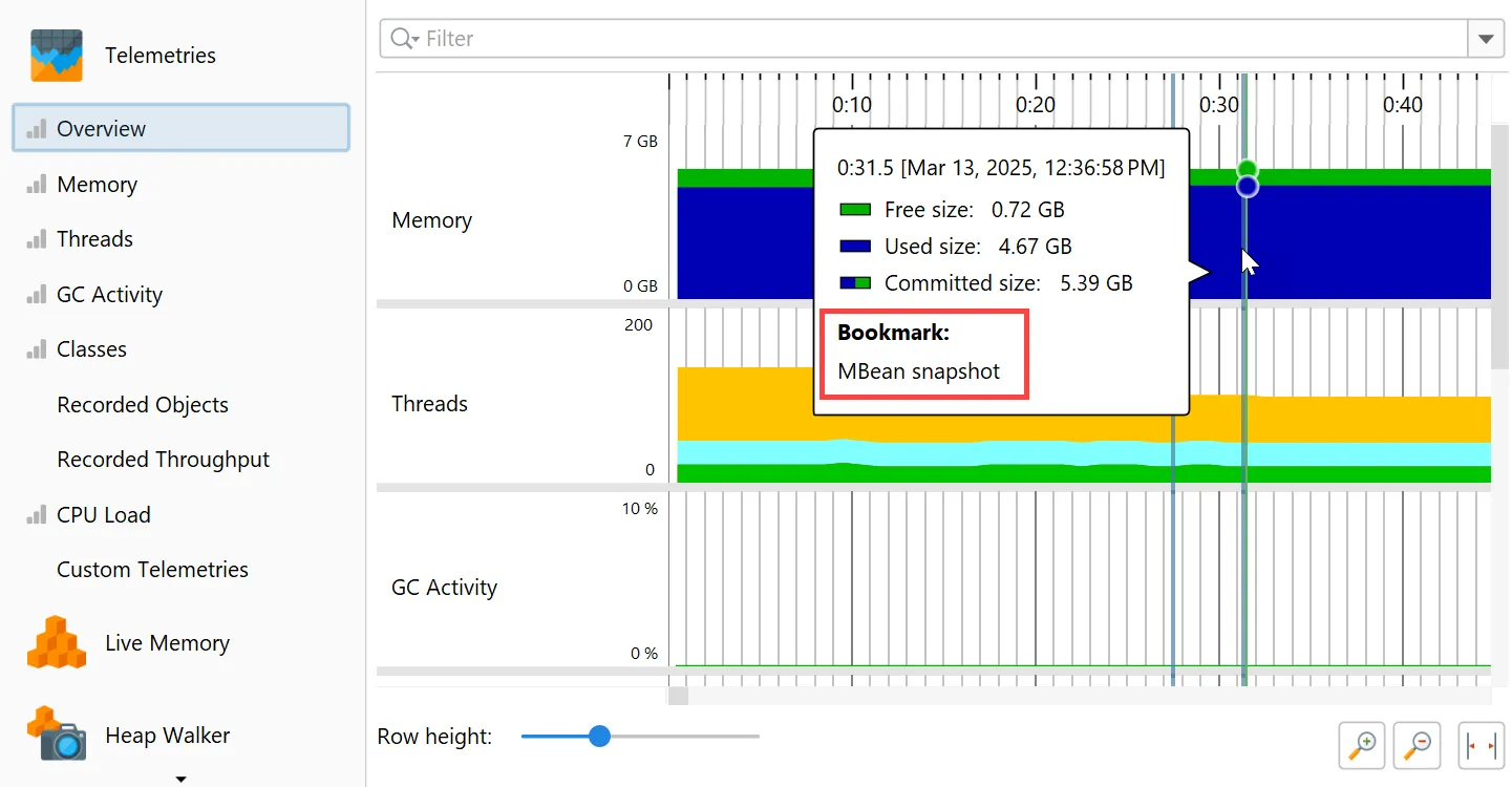
When you take an MBean snapshot, a bookmark is added to all views that have a time axis.
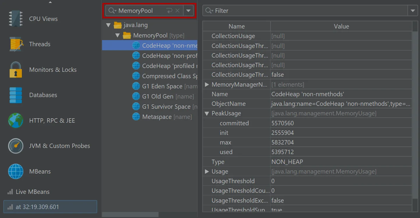
If you set a filter for the displayed MBeans, only the displayed subtrees will be included in the snapshot.
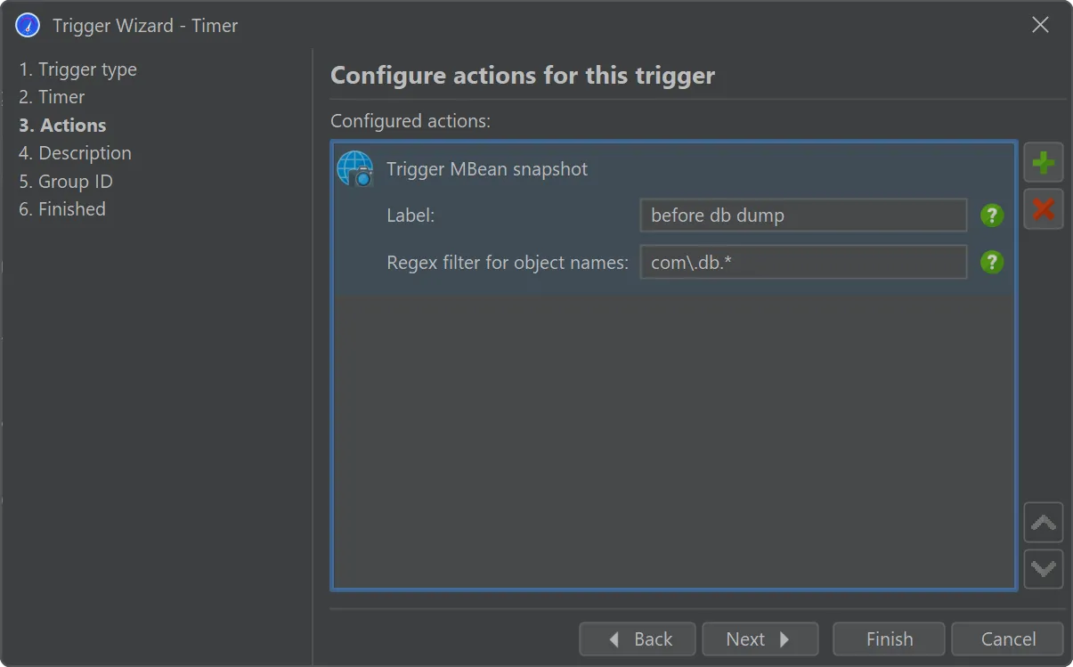
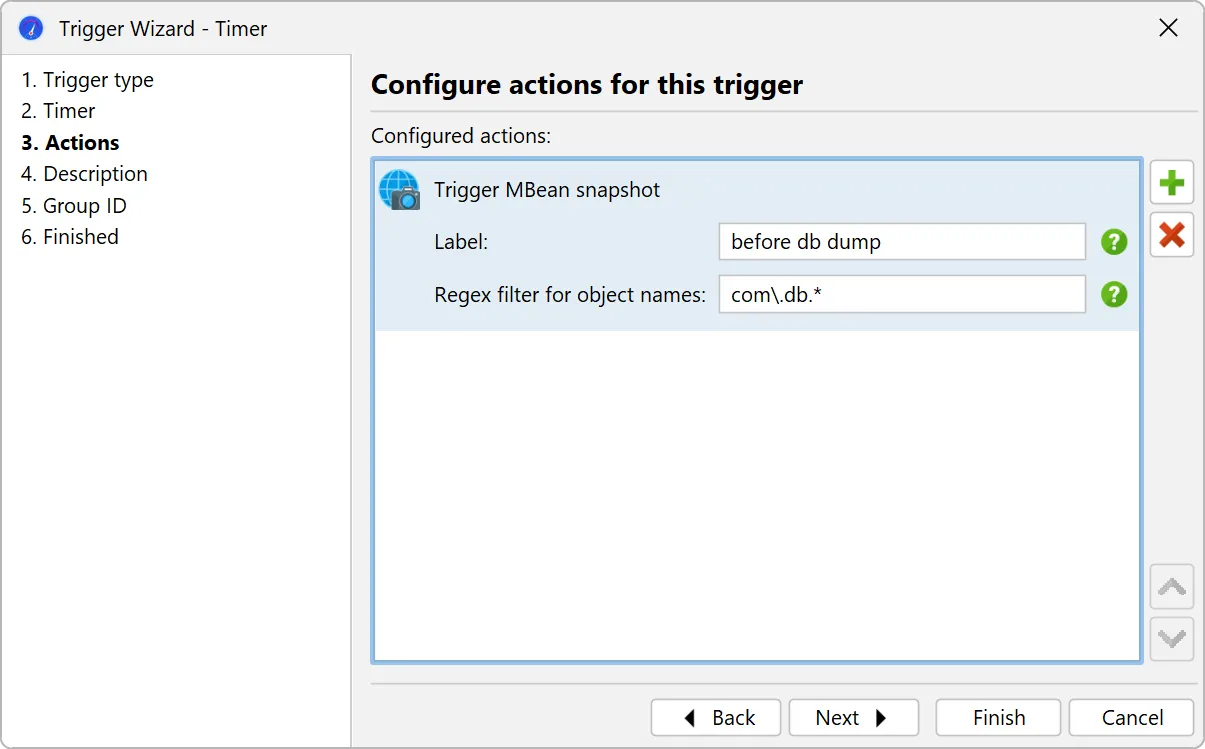
In the MBean snapshot trigger action, you can set a label as well as a filter for the included MBeans as well.
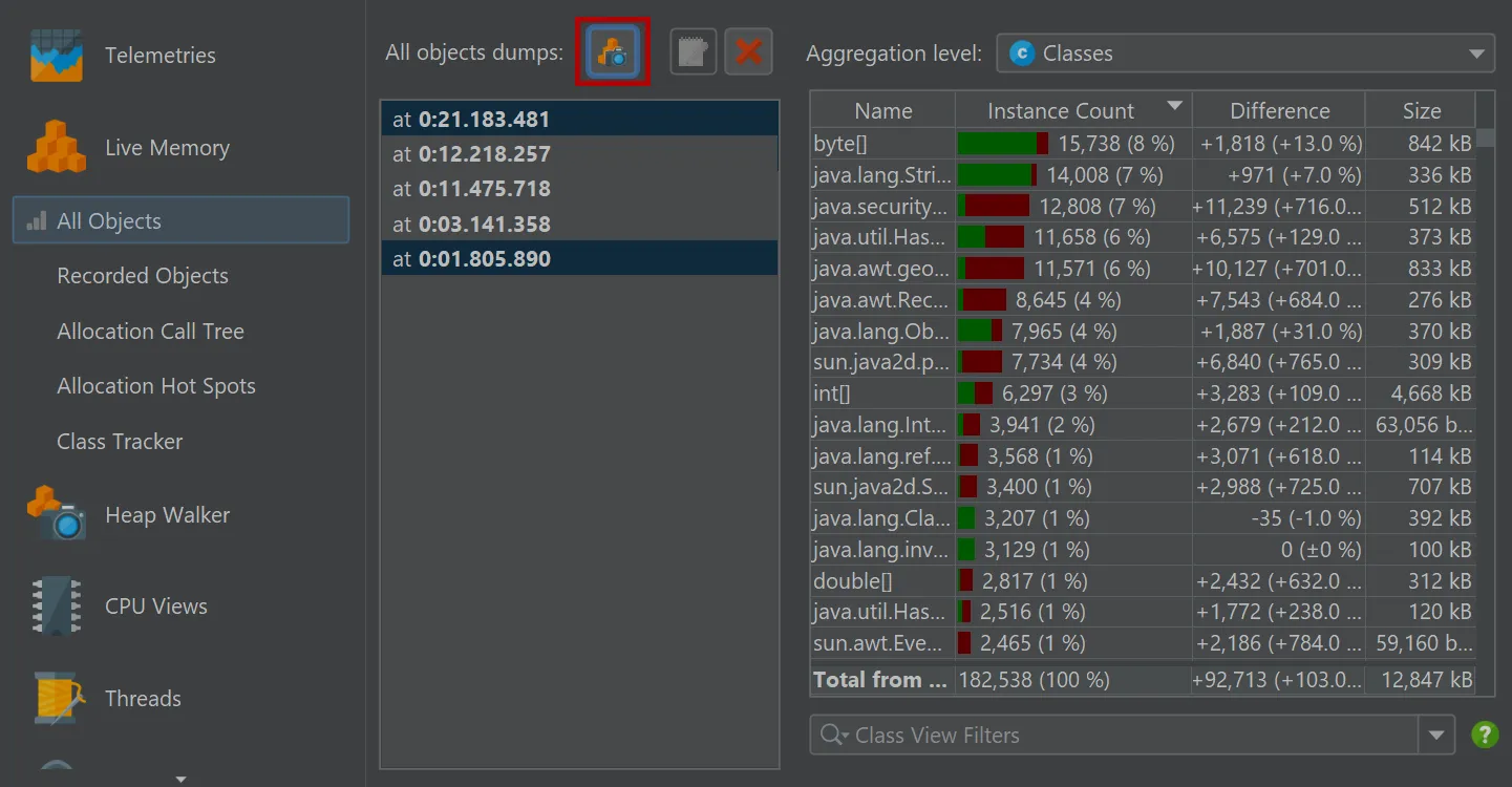
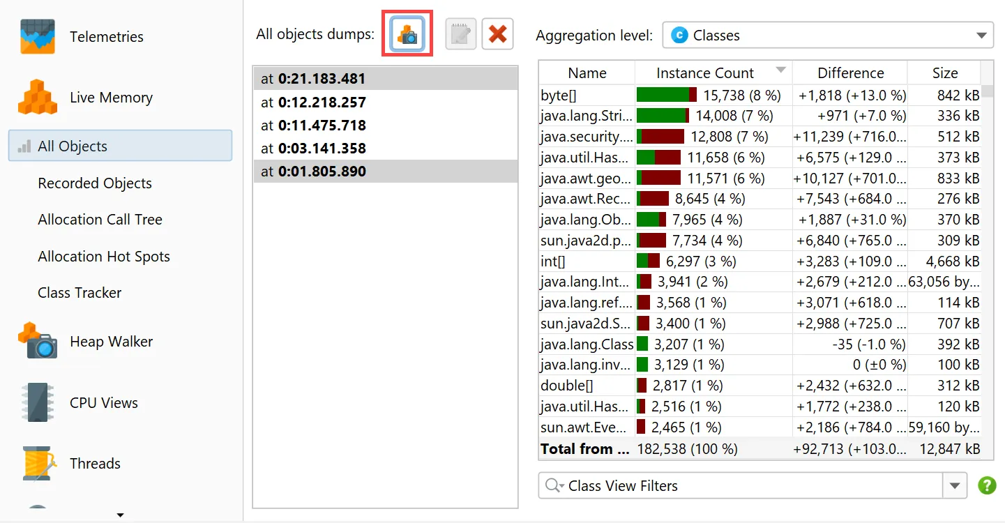
You can now take multiple "all objects" dumps.
The "All objects" view now has an action to take snapshots of the class histogram for all objects on the heap.
When two dumps are selected, the differences are shown in the view.
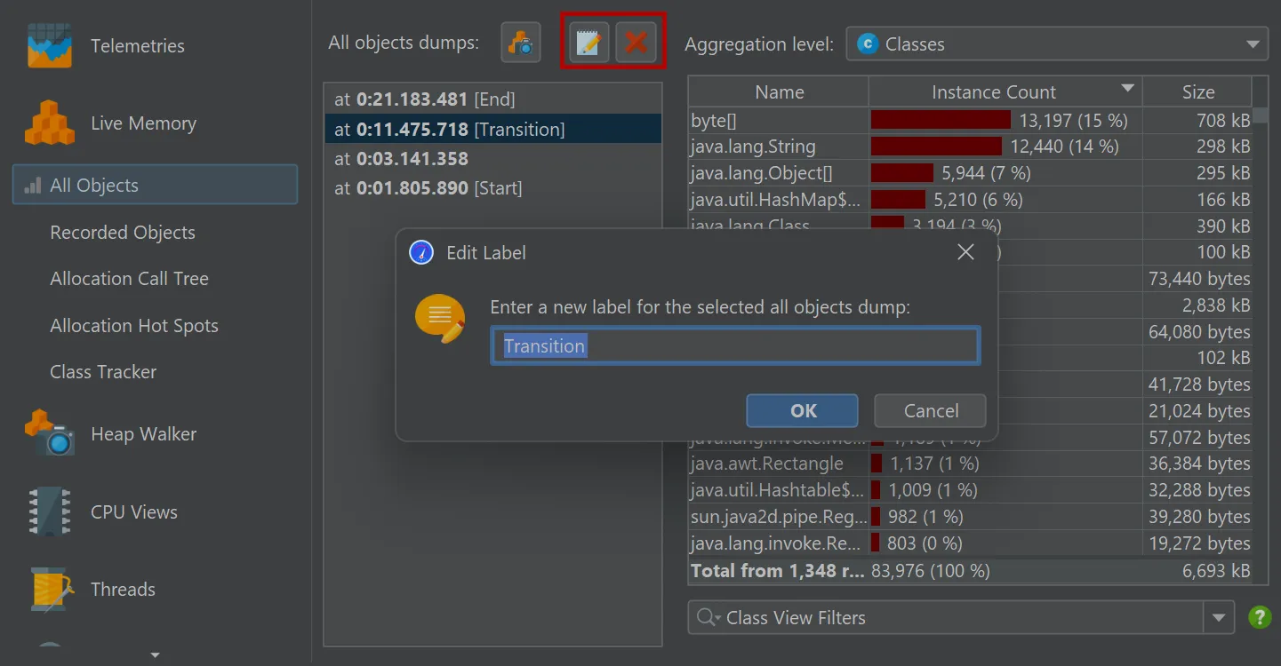
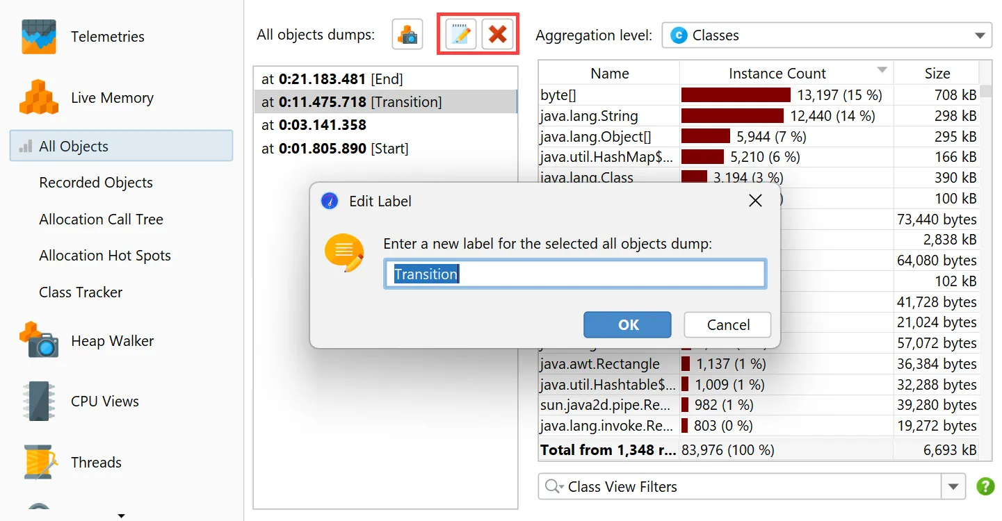
The toolbar above the dump selector offers actions to label and remove selected dumps.
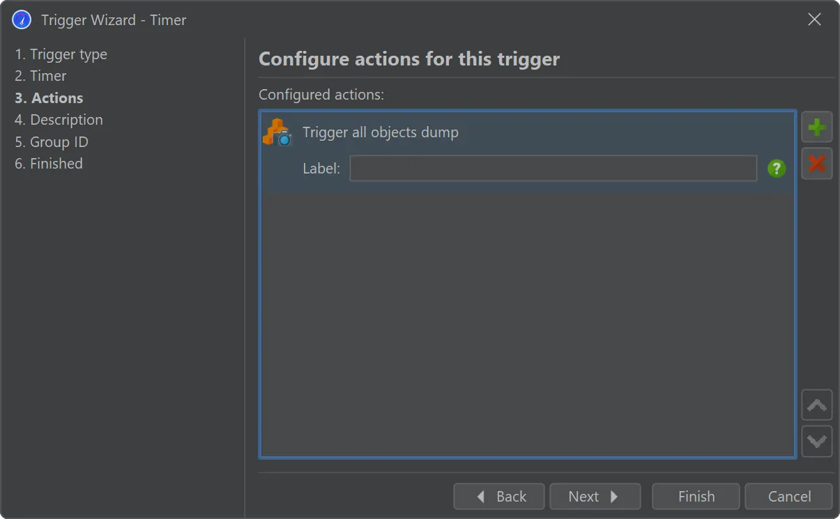
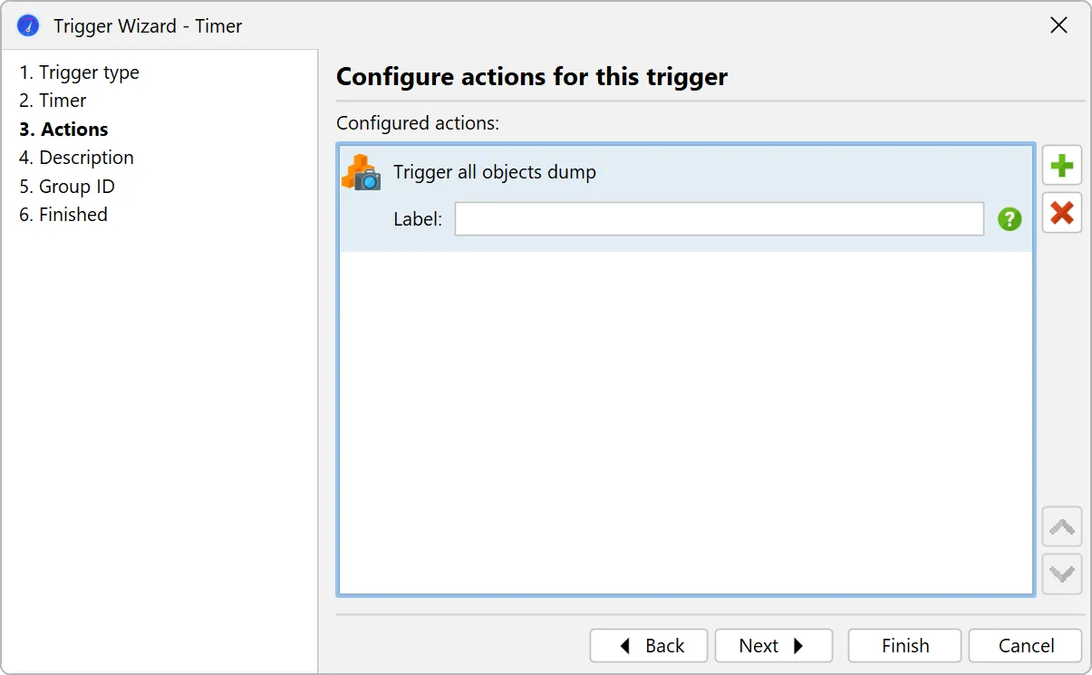
A trigger action has been added to take all object dumps programmatically, either in live mode or during offline profiling.
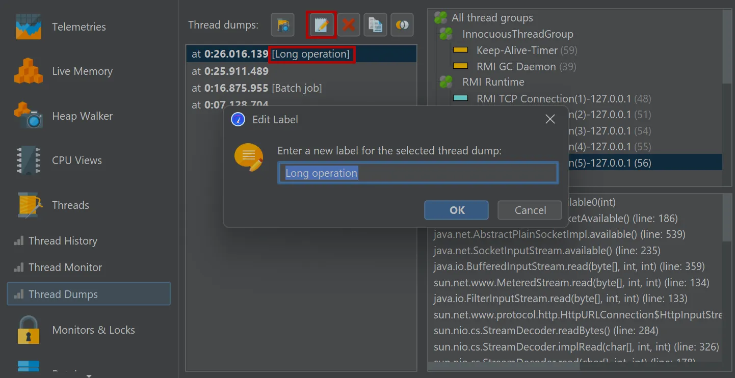
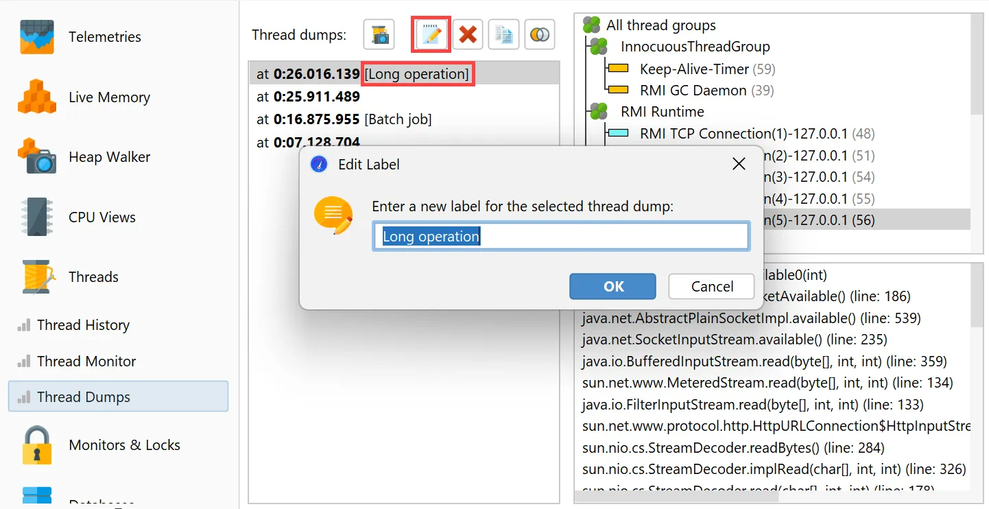
On a related note, it is now possible to label dumps in the thread dumps view as well.
This can also be done via the trigger action and the Controller API.
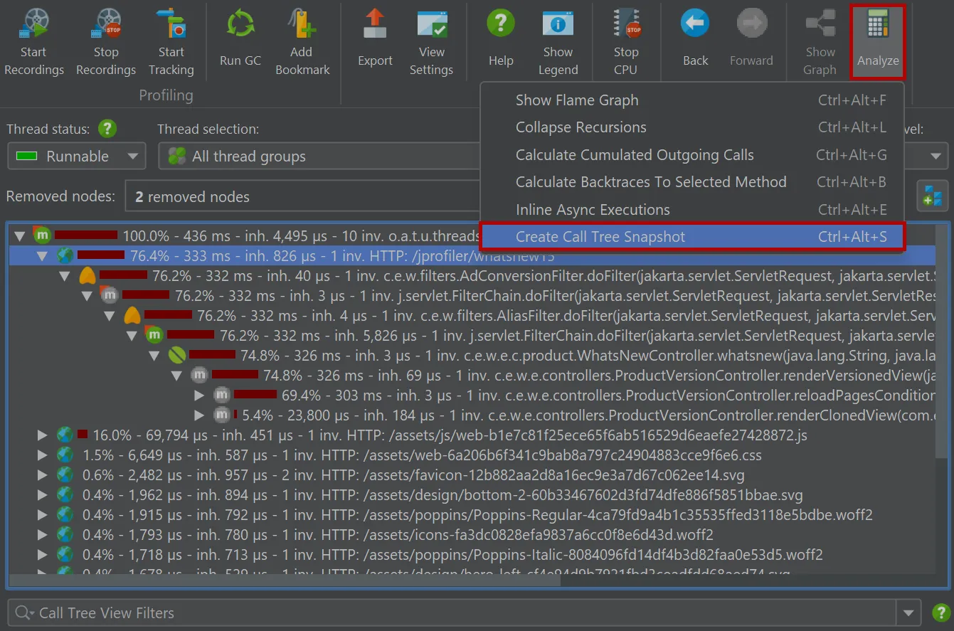
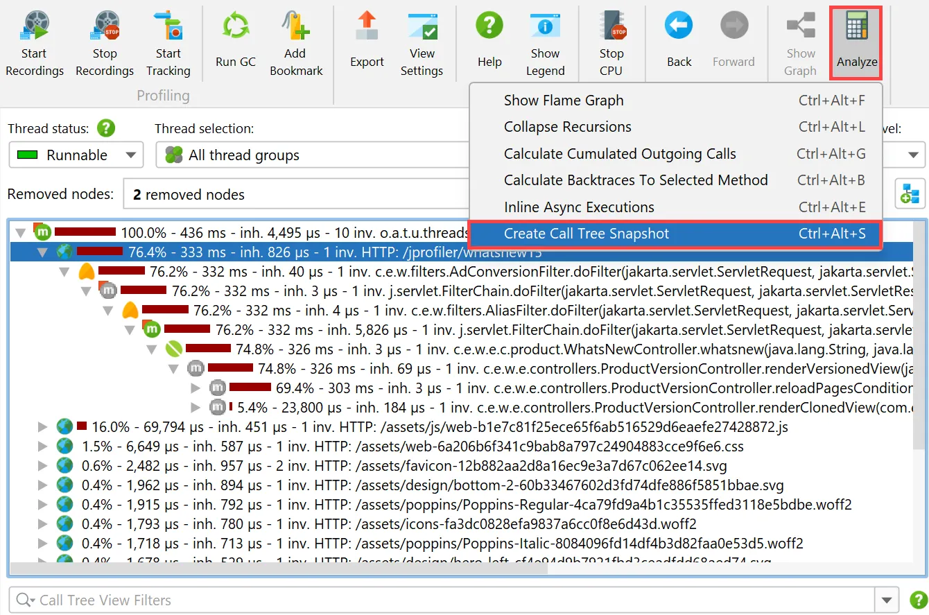
You can now make snapshots of the "Call tree" view in the CPU section.
For that purpose, a "Call tree snapshot" action has been added to the call tree analyses drop-down.
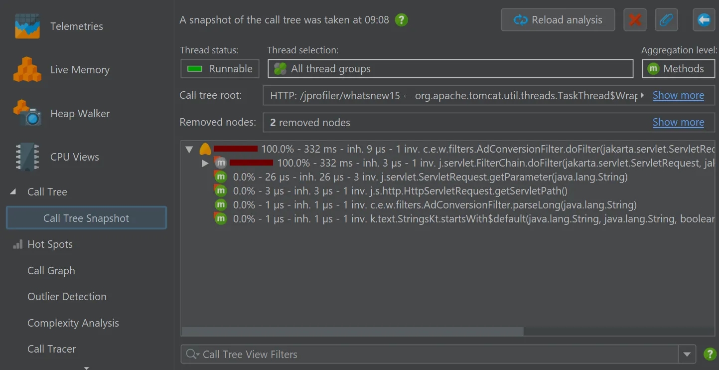
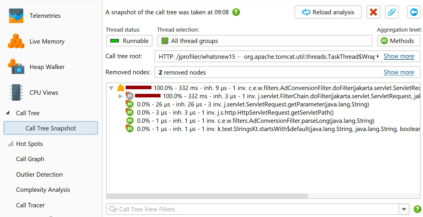
It creates a new call tree analysis view below the main call tree view that shows a static copy of the selected root, or the entire
call tree if no node was selected. All other view parameters like thread status or aggregation level are fixed in the call tree snapshot.
Unlike other call tree analyses, call tree snapshots are saved into JProfiler snapshots, because they contain separate data.
With this tool, you can manage different call tree recordings without resorting to saving full snapshots that you have to open in
different JProfiler windows. Instead, you can remain in the same live session and keep different sets of recording data around.
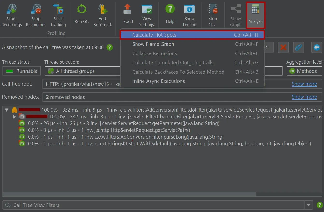
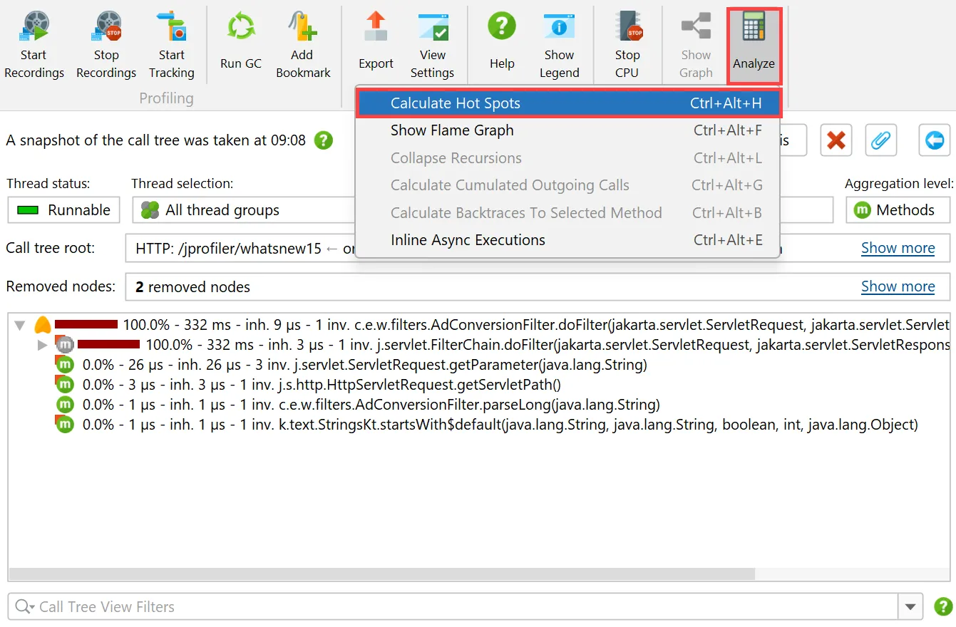
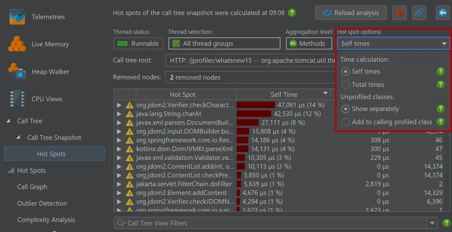
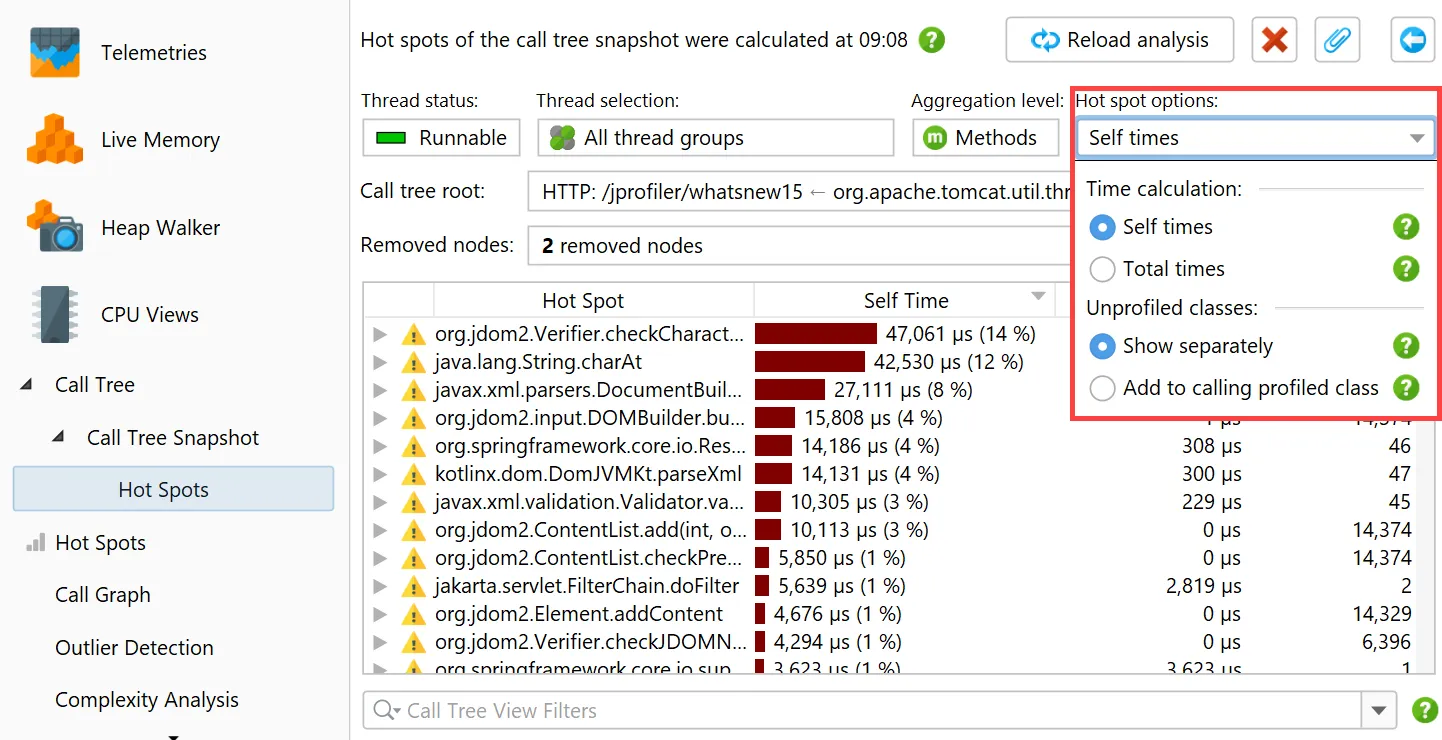
In the call tree snapshot view, a "Calculate hot spots" analysis action is available besides the usual call tree analysis types.
The resulting hot spot view is added as a child of the call tree snapshot view and shows the static hot spots for the data in the parent
view. The hot spot calculation options are still adjustable here.
Call tree analyses have been improved.
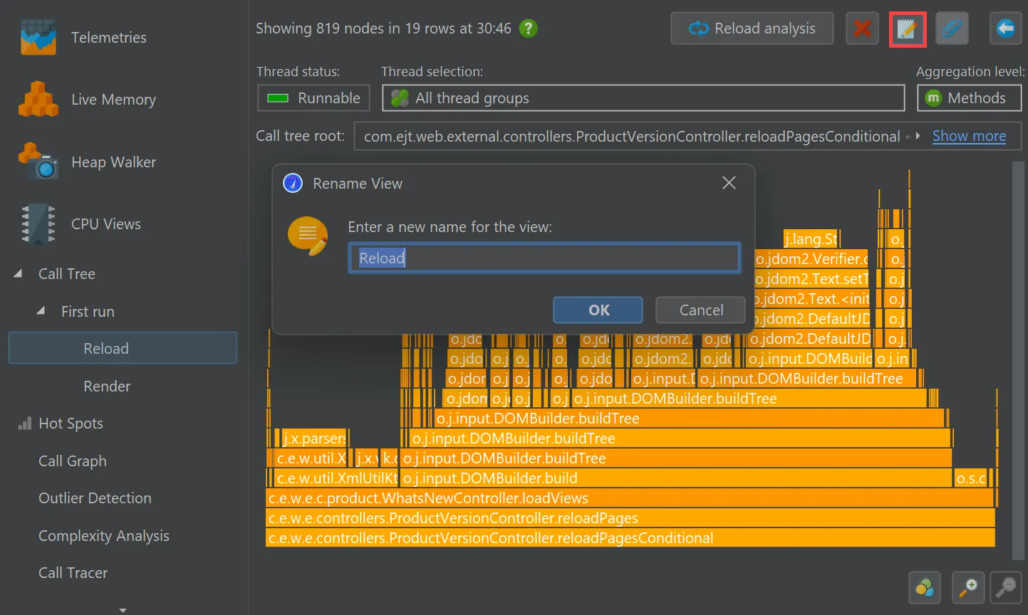
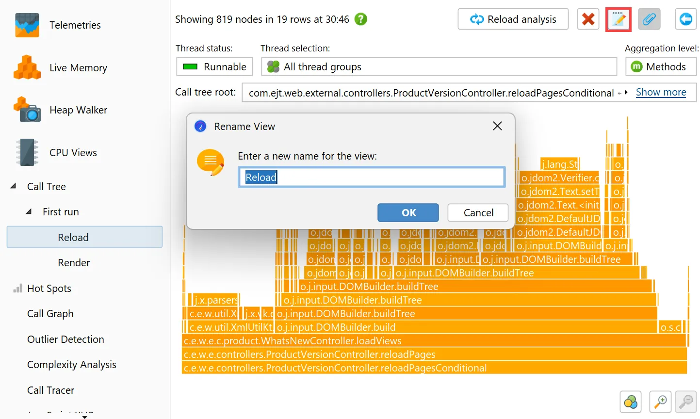
You can now rename call tree analyses. After making them permanent with the pin button, a rename button will appear that changes
the name of the analysis in the view selector.
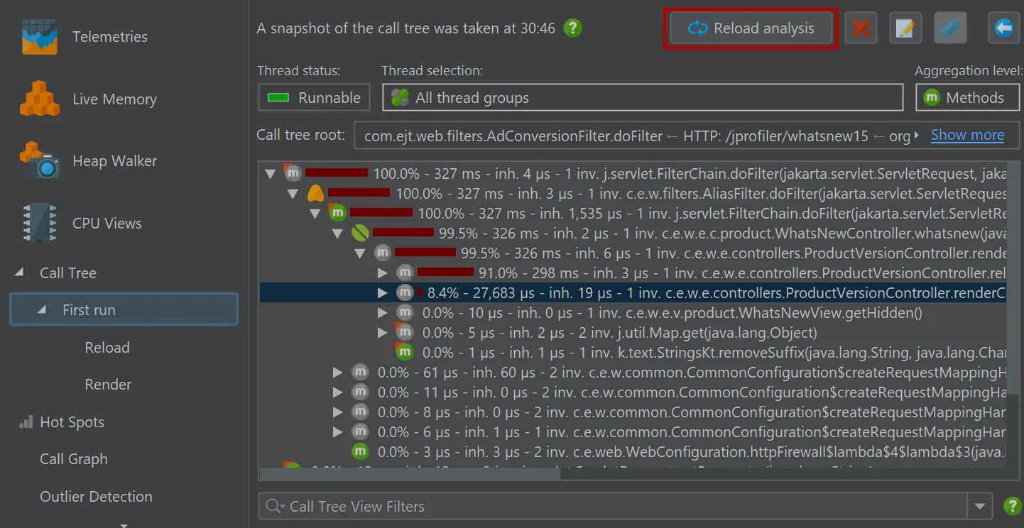
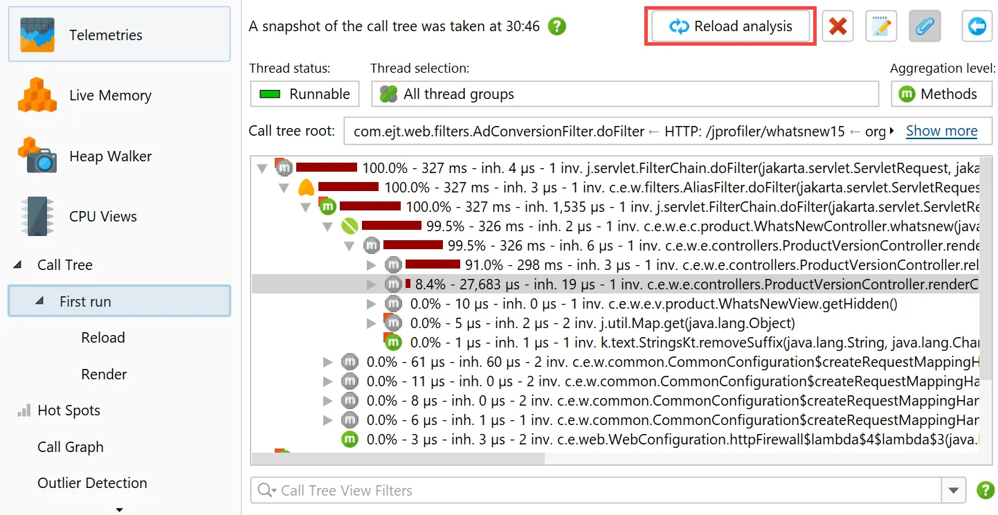
In addition, the "Reload analysis" button goes back to the top level ancestor view and re-calculates all ancestor views
and all descendant views for the new data. In the example below, the current data in the live call tree would be used to update the
call tree view labeled "First run" and then the flame graph views labeled "Reload" and "Render".
Heap walker filter and grouping scripts on dumped data have been added.
Previously, only filter and grouping scripts on live objects were available which did not work for snapshots. Also, changing data
and garbage collection of objects may require operations on dumped data instead of live data.
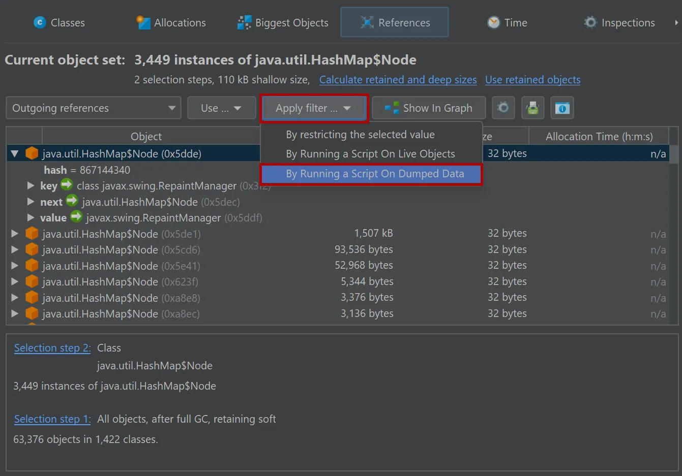
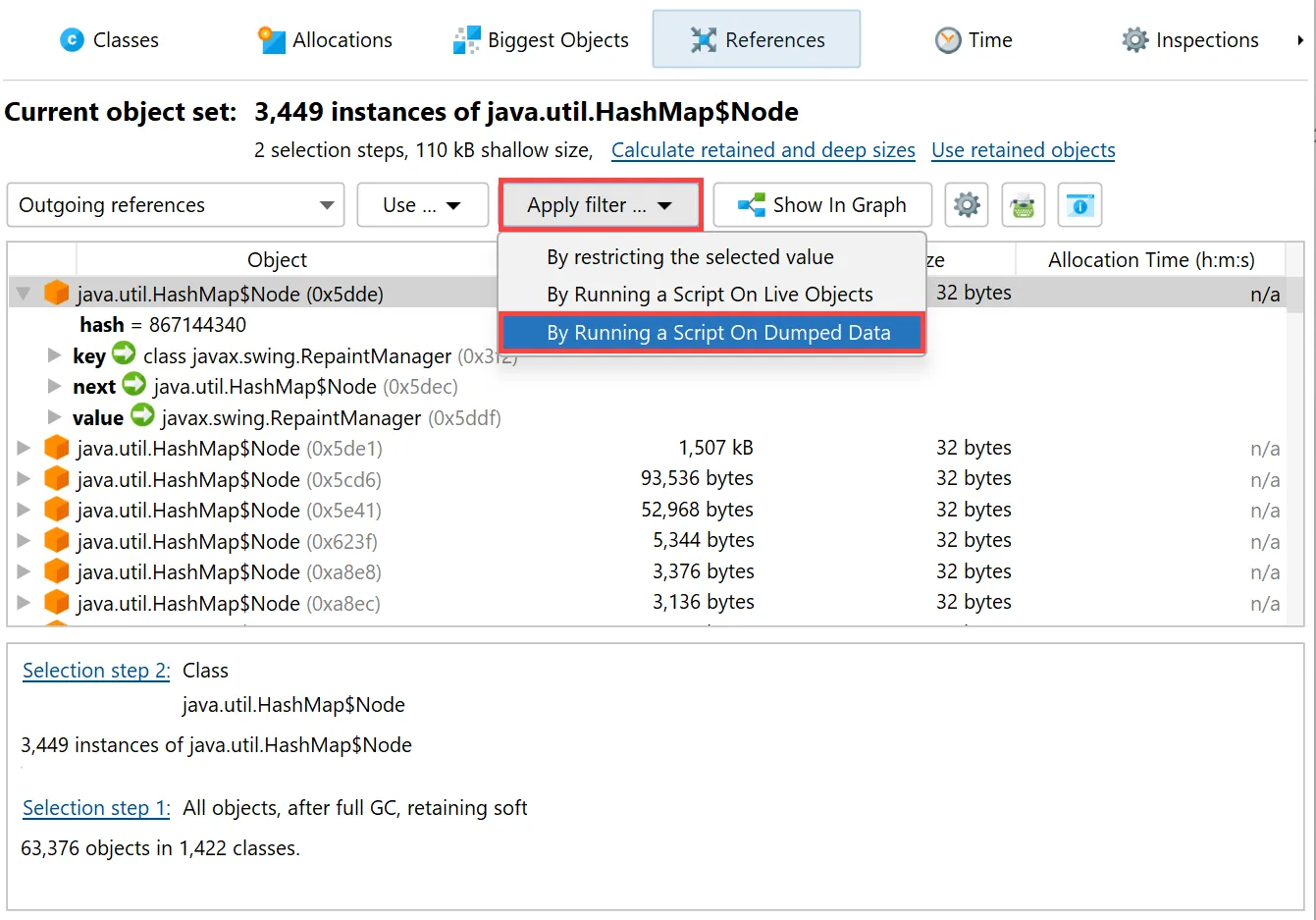
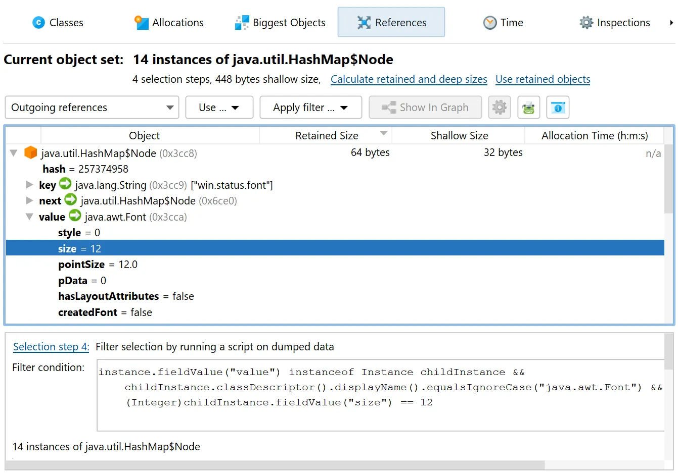
In the references view of the heap walker, the "Apply filter" dropdown contains a new action to filter objects by running a script on
dumped data.
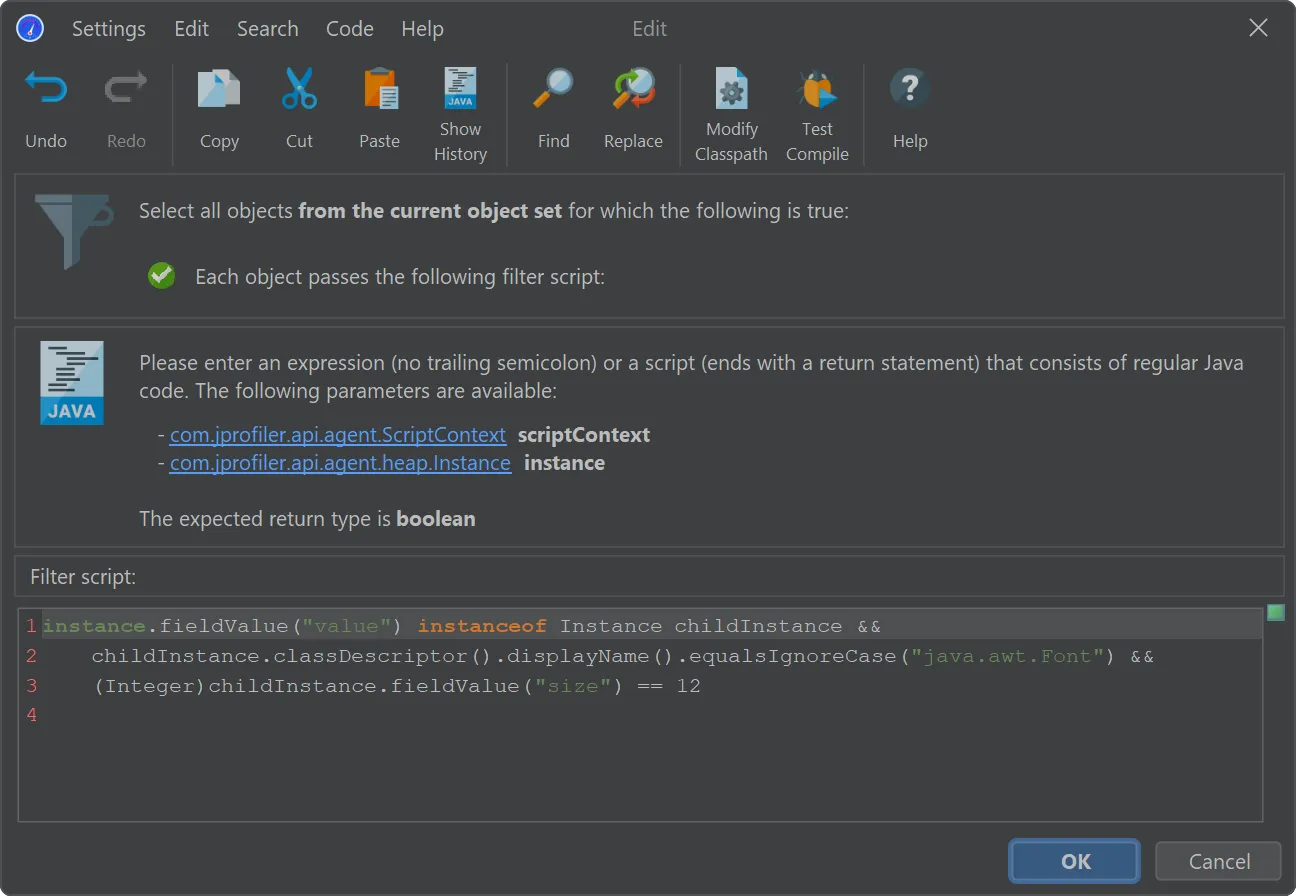
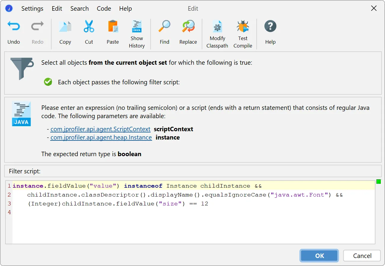
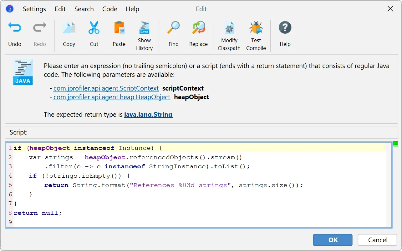
In the script editor, objects from the com.jprofiler.api.agent.heap API are passed as an argument, and the boolean return value
of the script decides whether the object is included in the new object set.
In general, the parameter is of type com.jprofiler.api.agent.heap.HeapObject but can be narrowed to a subtype if the current
object set allows it. In the screenshot below, the current object set only contained java.util.HashMap$Node instances, so the
parameter is of type com.jprofiler.api.agent.heap.Instance which provides access to field values.
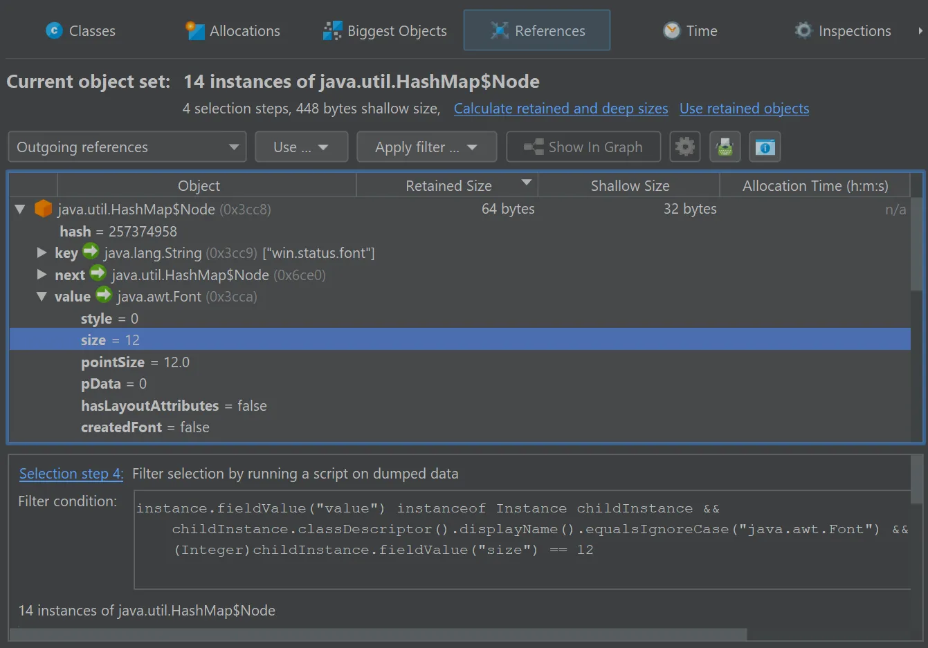
The script selects java.util.HashMap$Node instances whose value is a java.awt.Font with a size of 12.
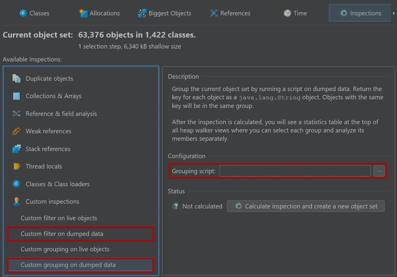
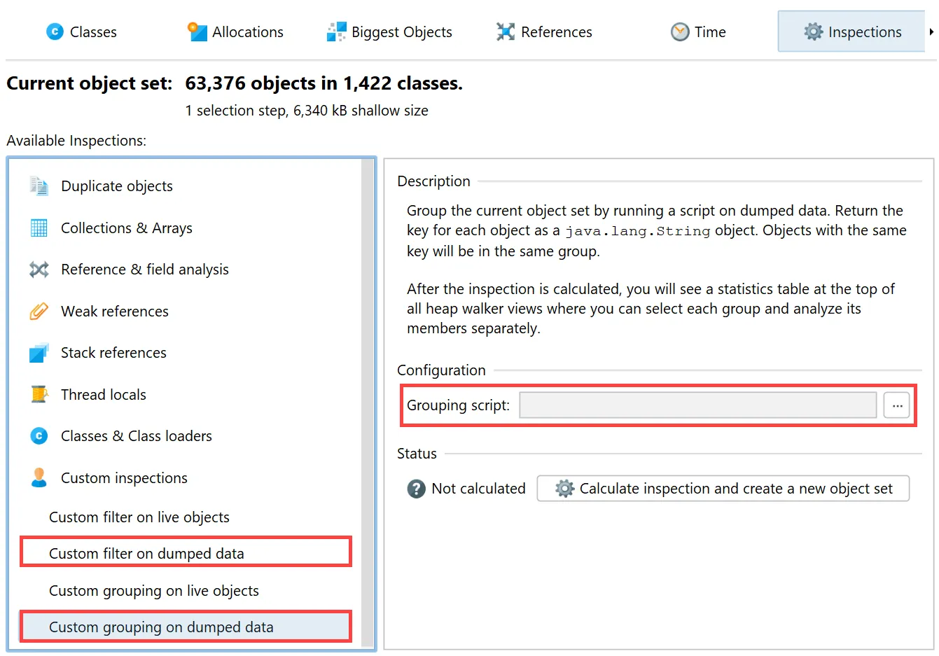
In addition to the filter script in the references view, JProfiler provides an inspection to filter all objects in the current
object set as well an inspection which groups all objects according to the string return value of a script.
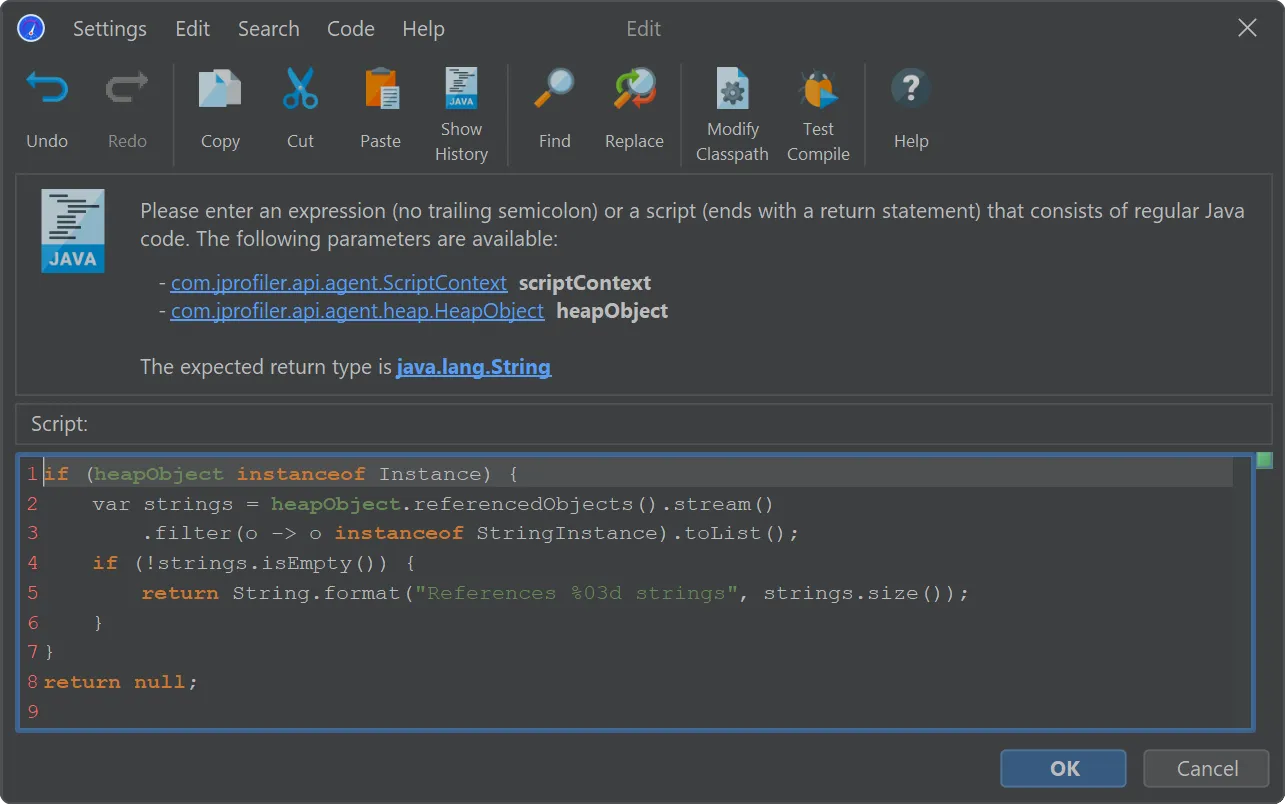
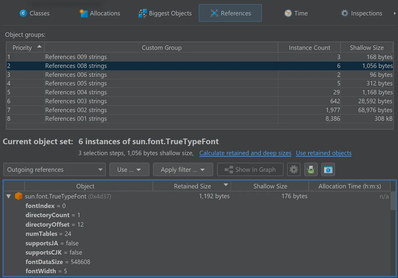
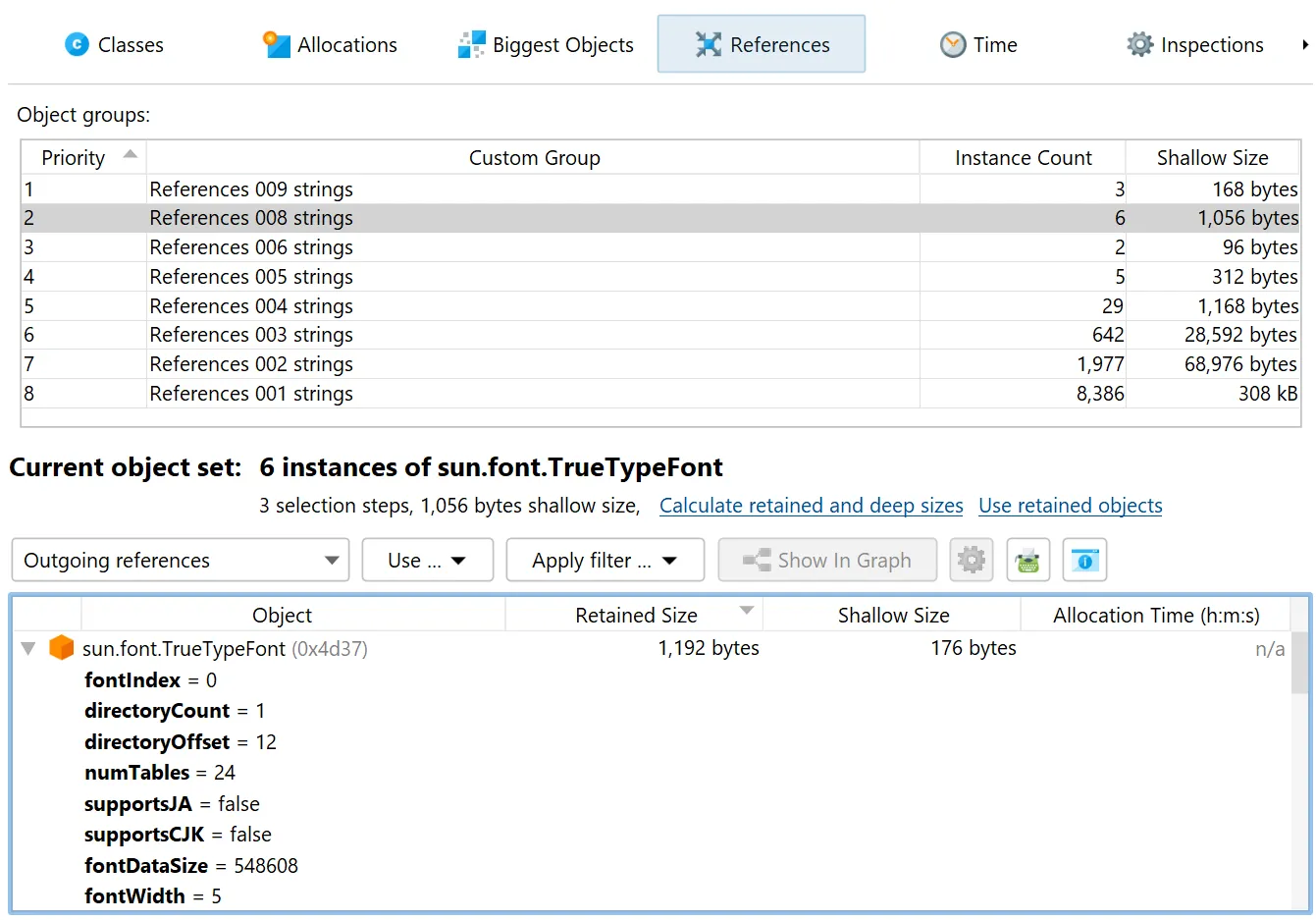
In the "Custom grouping on dumped data" script below, all regular instances are grouped by the number of strings that they reference.
If the passed object is not a regular instance or if it does not reference any strings, the script returns null and the object
is not included.
As for other kings of groupings, a grouping selector is shown at the top after the inspection has been calculated. When you select a group
row, the current heap walker view will only show the instances that are contained in that group.
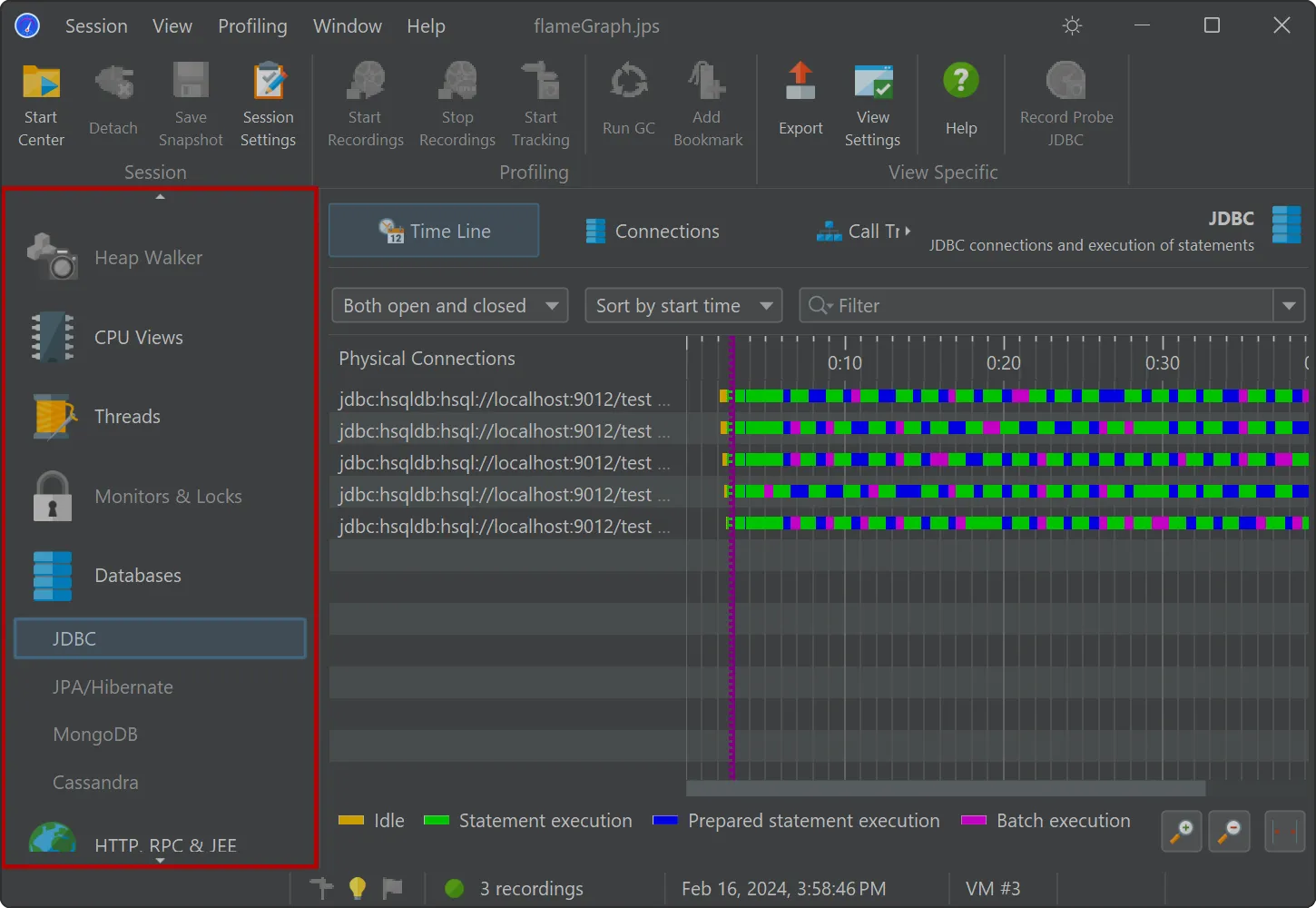
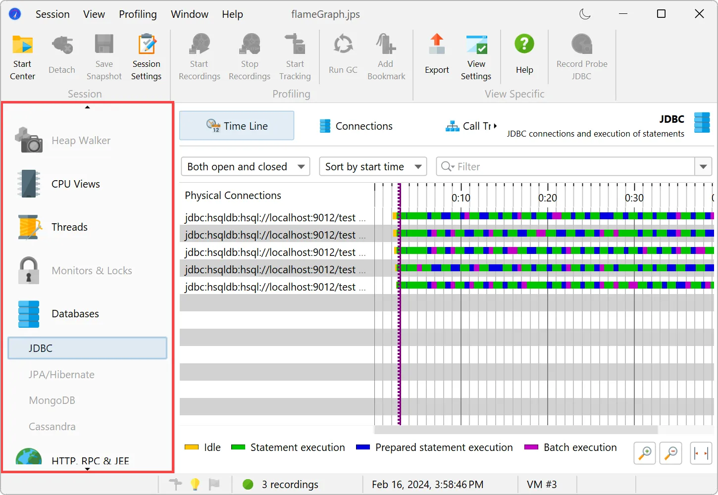
JProfiler 15 makes it easier to see which views contain data.
For snapshots, all views without recorded data are now shown as disabled in the view selector.
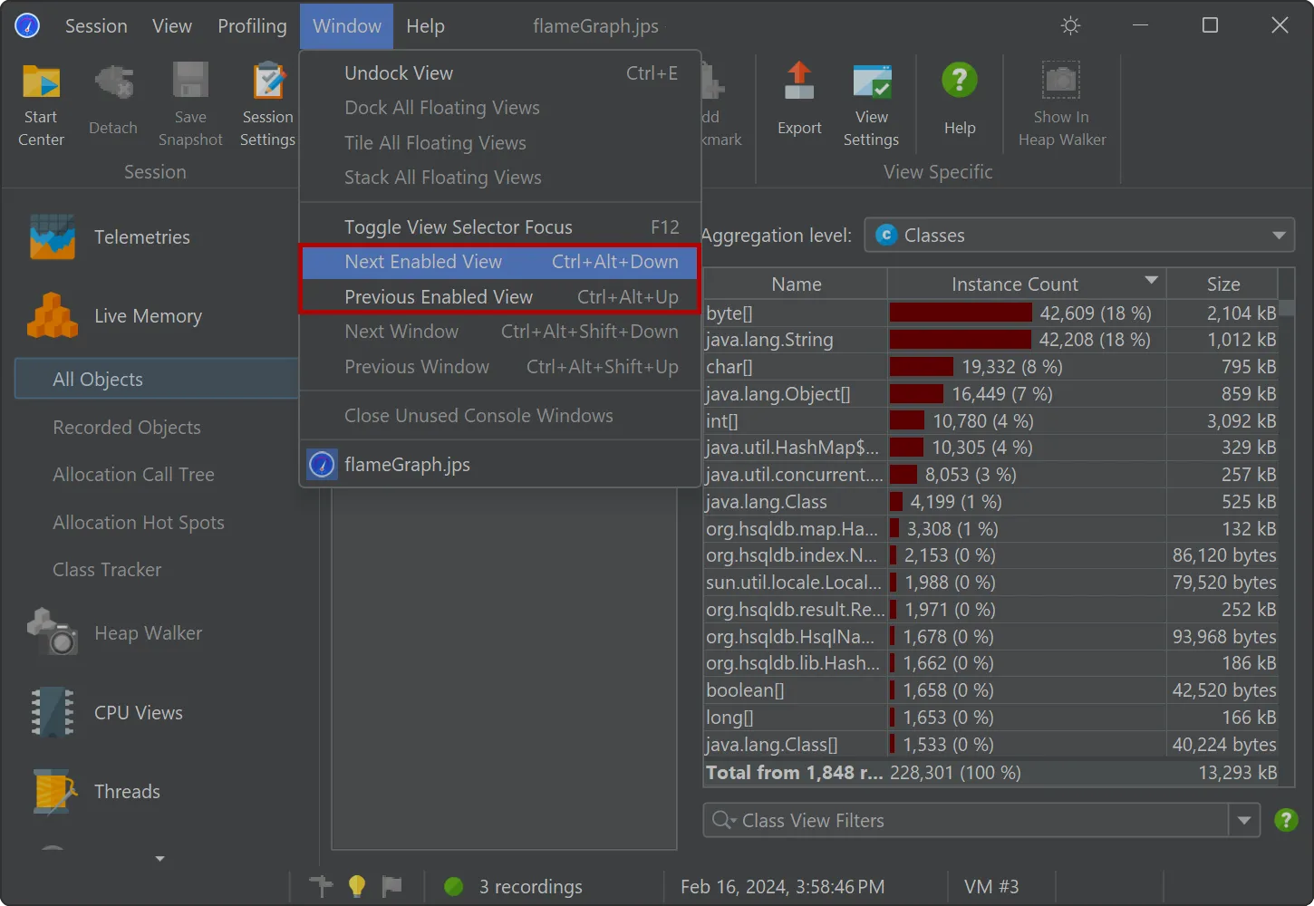
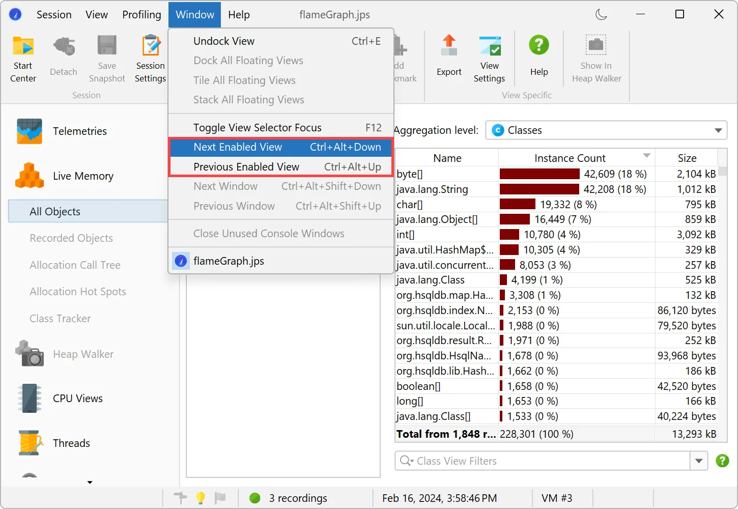
With the new "Next enabled view" and "Previous enabled view" actions, you can quickly step through all relevant views.
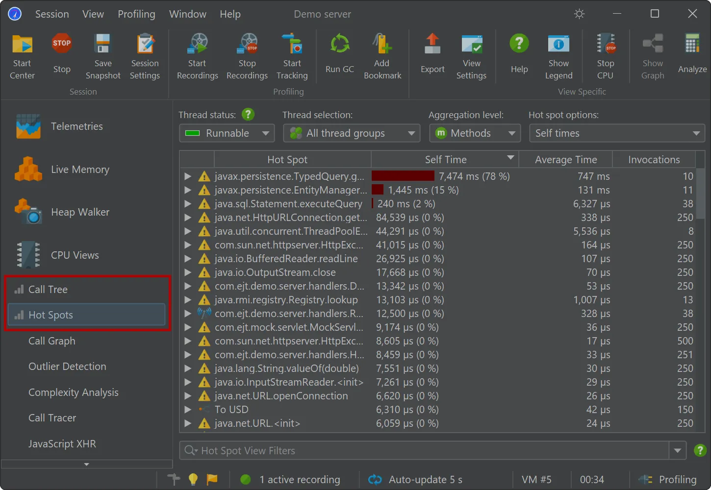
For live sessions, the views displaying recorded data now have a special marker in front of the view name.
A Japanese locale has been added. こんにちは、日本!
The UI as well as the documentation have been fully localized into Japanese.
The language can be changed in the general settings and will be auto-detected by the installer.
A Korean locale has been added. 안녕하세요, 한국!
The UI as well as the documentation have been fully localized into Korean.
The language can be changed in the general settings and will be auto-detected by the installer.
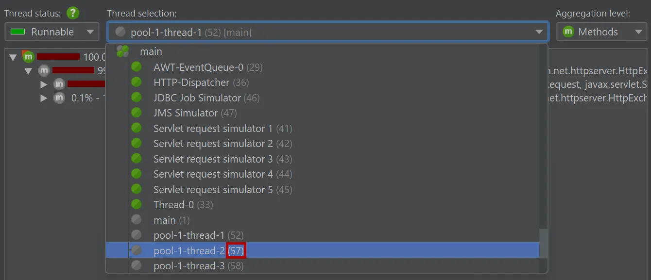
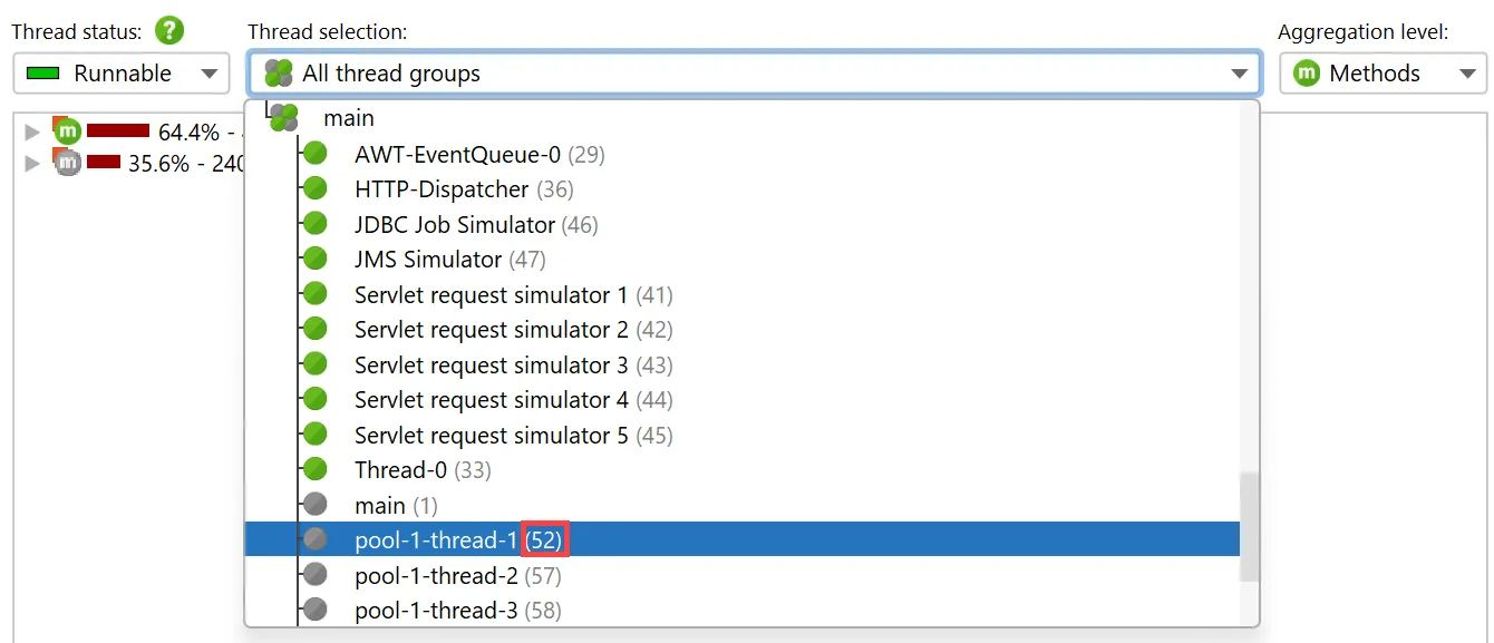
Thread IDs are now shown in the UI.
Previously, only thread names were displayed which are not necessarily unique. Now the unique ID of each thread is added, so that
you can identify particular threads under all circumstances.
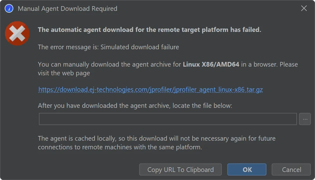
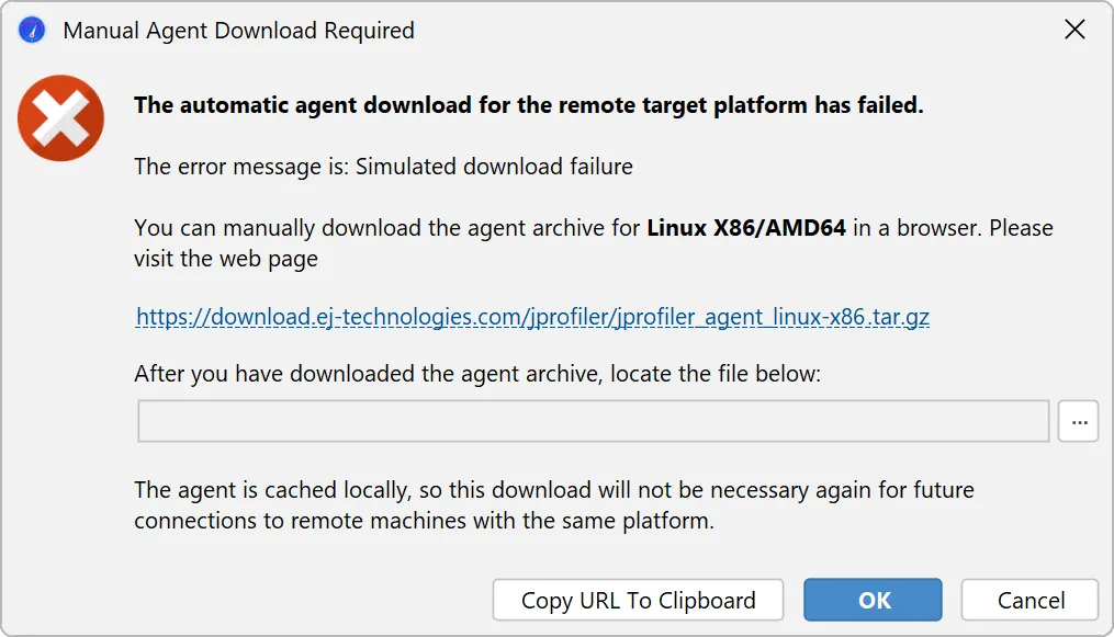
The process for handling a download failure of JProfiler agent archives for remote profiling has been improved.
During a zero-configuration remote attach operation, JProfiler needs to upload the profiling agent for the remote platform.
If the agent for the remote architecture is not available, JProfiler will download and cache it locally. In the case of restrictive
firewalls, such a download may not be possible.
While previous workarounds were cumbersome, JProfiler 15 now offers a workflow for procuring the agent archive with a browser and
telling JProfiler about the externally downloaded archive.
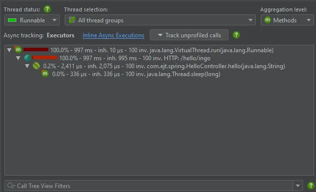
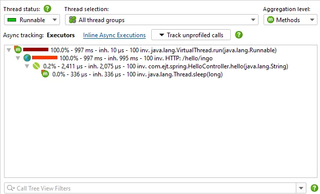
JProfiler 14 adds full support for profiling Java 21, including virtual threads.
Java virtual threads are thread-like tasks that aim to revolutionize high-scale concurrency on the JVM.
All aspects of JProfiler have been reworked so that profiling millions of virtual threads causes minimal overhead.
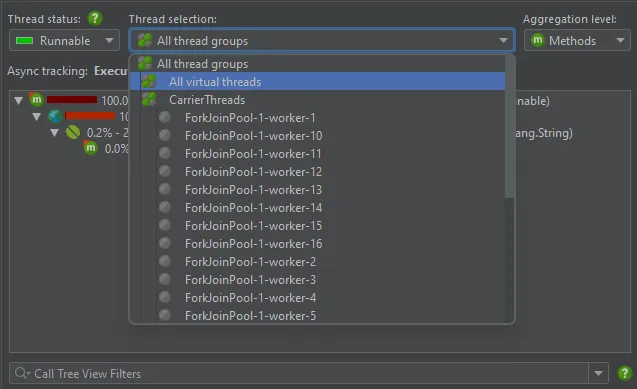
In the call tree, virtual thread executions will have a top-level node of java.lang.VirtualThread.
Virtual threads are not recorded separately like platform threads, so all virtual threads are contained together in a single synthetic
thread group.
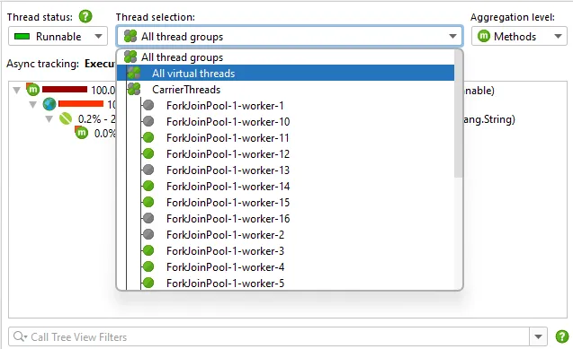
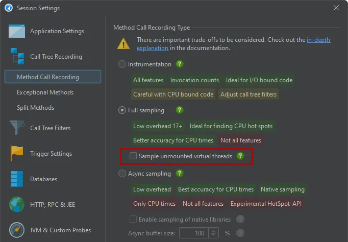
By default, only mounted virtual threads are sampled. This means that blocking states of virtual threads are not captured by CPU recording.
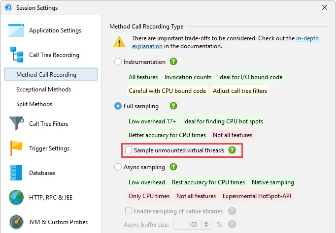
For debugging purposes, there is an option in the profiling settings to sample unmounted virtual threads.
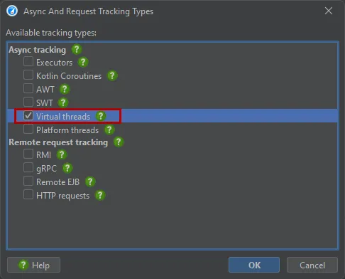
Like for platform threads, JProfiler supports async tracking for the creation of new virtual threads. If enabled, the
"Inline Async Executions" call tree analysis connects call sites with execution sites. In this case, the call site is the last profiled
method before the VirtualThread instance is created. The execution site is a top-level node in the started virtual thread.
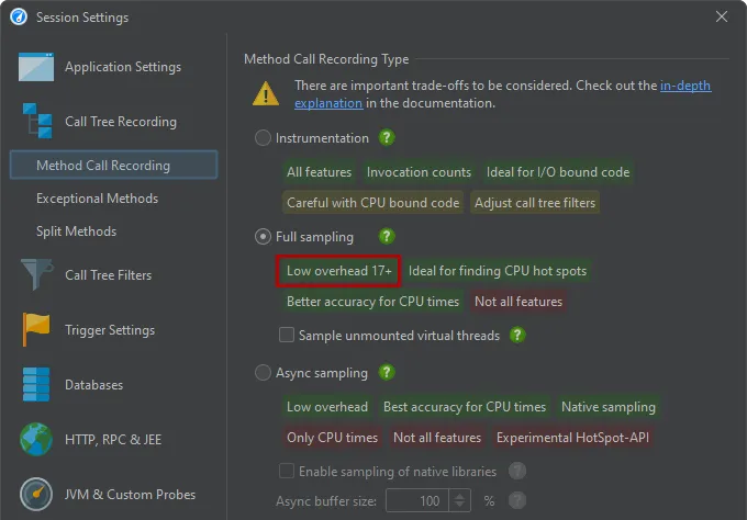
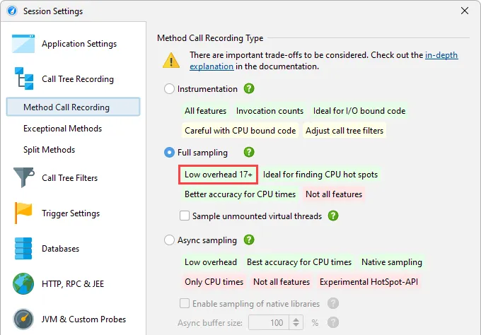
Near-zero overhead for full sampling when profiling Java 17+. Using new facilities in the JVM, JProfiler can now perform sampling
with a negligible overhead, even for heavily multi-threaded applications where the overhead for sampling used to be significant.
From an overhead perspective, sampling is now on equal terms with async sampling if you profile Java 17 or higher.
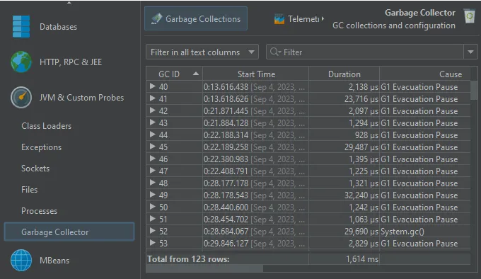
A garbage collector probe was added. The GC probe is available when profiling Java 17+ and shows detailed data about single garbage
collections and the GC configuration.
Because of the increasing number of probes, the probe sections have been reorganized and the GC probe can be found in the new
"JVM & Custom Probes" section.
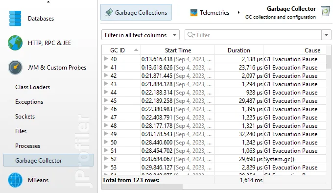
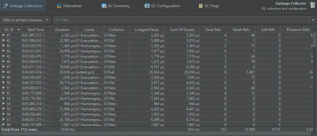
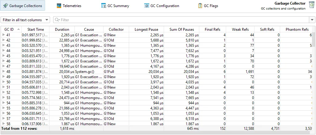
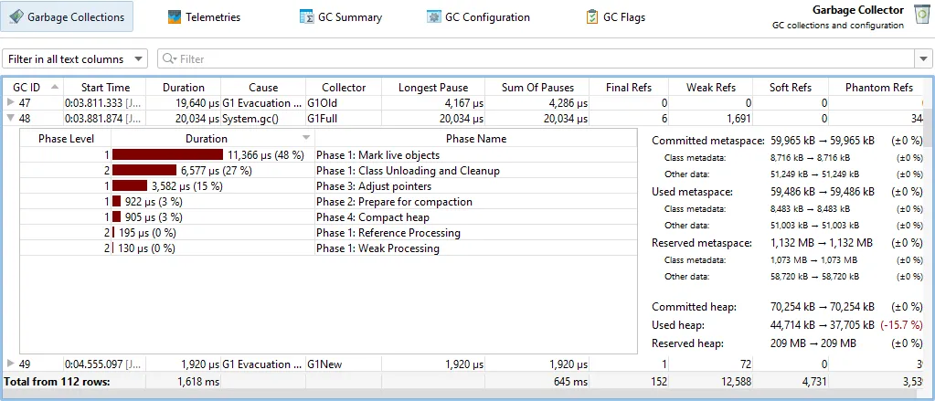
Its main view is the "Garbage collections" view that shows single garbage collections in tabular form. It shows you the triggering cause,
how long the collection took, how many references were collected and what pauses were caused by the garbage collection.
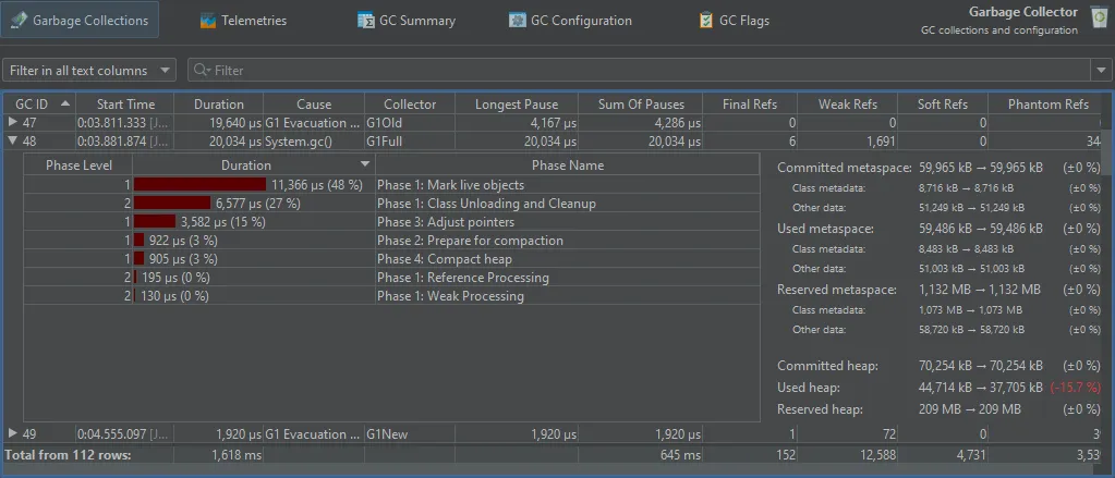
If you need even more detail, each garbage collection can be expanded to show the single phases with their duration. To the right of the
GC phase table, statistics about the changes in heap and metaspace are shown.
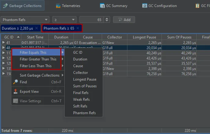
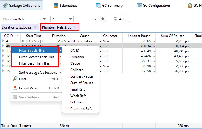
To help you analyze important garbage collections, you can set multiple filters, most conveniently with the context actions on the
garbage collections table and the phase table. Filters are added as tag labels above the table and can be removed by clicking their close button.
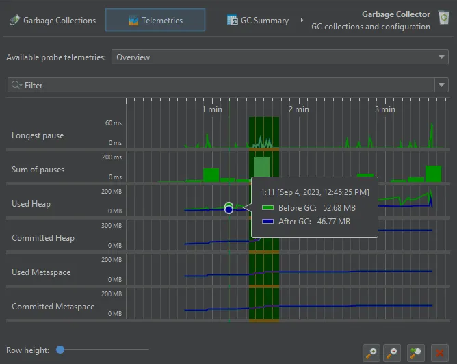
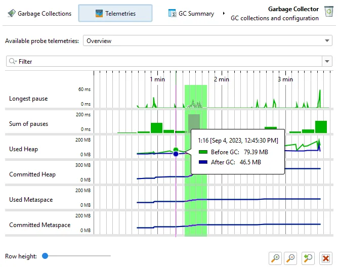
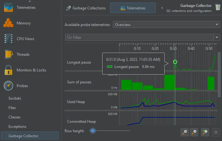
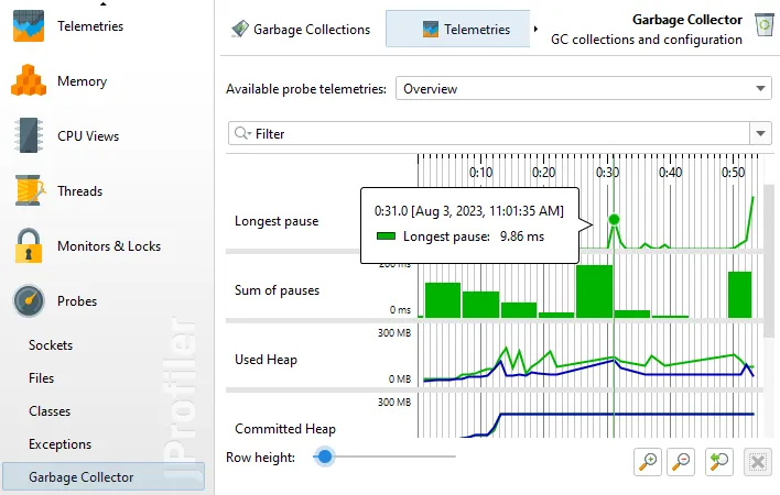
The GC probe produces a number of GC telemetries which are available in the "Telemetries" probe view.
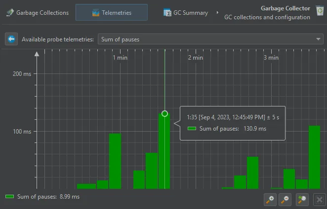
If you are interested in minimizing GC pauses, the "Longest pause" telemetry at the top will be the most interesting one.
You can drag along the time axis of the telemetry to select the corresponding garbage collections in the "Garbage Collections" view.
For better vertical resolution, you can select a single telemetry from the drop-down at the top or by clicking on the name of the telemetry.
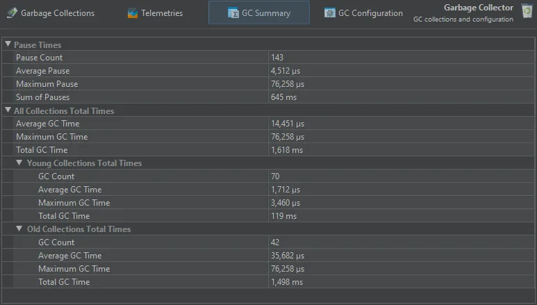
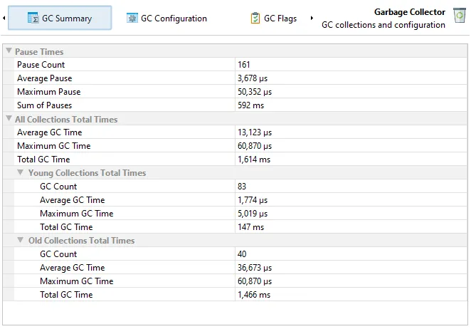
The GC summary view shows you measurements that are aggregated over the entire recording period. Each measurement provides the number
of garbage collections, as well as the average, maximum and the total values. The most important data at the top are the "Pause times"
that directly affect the liveness of your application.
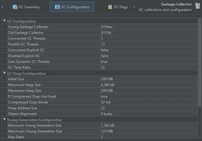
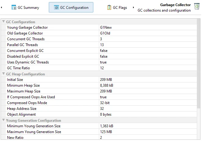
In the GC configuration view, you can inspect the common properties that can either be set explicitly or that are set
implicitly by the garbage collector itself. These properties are common to all garbage collectors and help you understand the
differences between garbage collectors.
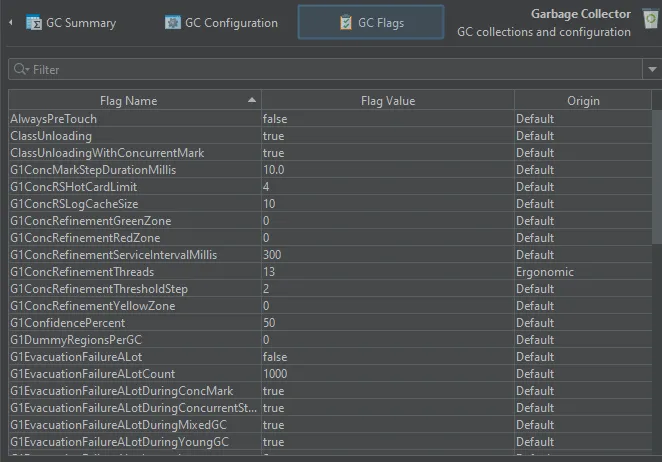
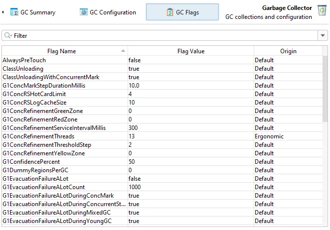
Finally, the GC flags view gives you an idea what properties of a garbage collector can be tuned and lets you check their actual
values. The "Origin" column shows you how the flag was set.
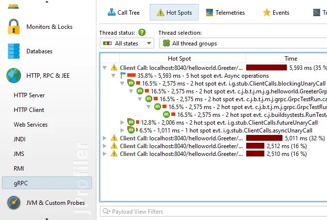
A gRPC probe has been added. gRPC is a popular RPC framework that uses HTTP/2 and Protocol Buffers, offering features like
streaming and multiplexing. This probe can be found in the new "HTTP, RPC & JEE" probe section.
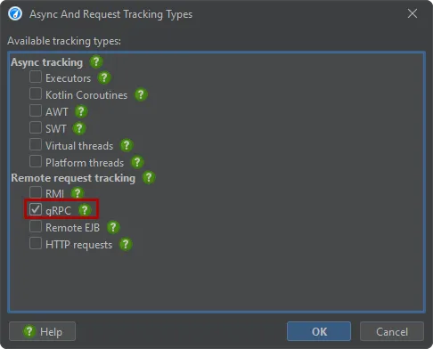
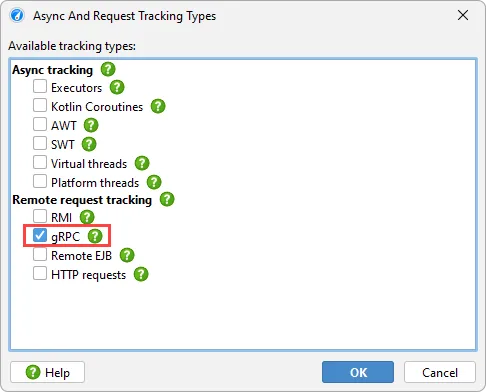
JProfiler can track remote gRPC calls between JVMs if gRPC remote request tracking is enabled.
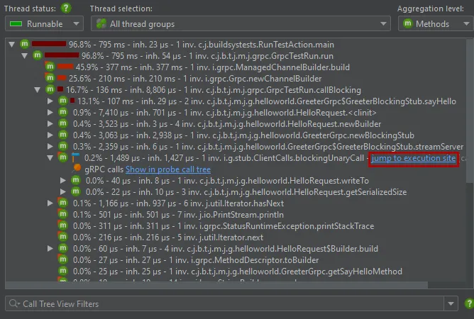
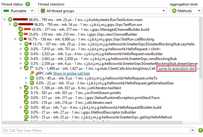
You can then see hyperlink labels in the call tree view for incoming and outgoing calls that will take you to the corresponding
call tree location. This requires that both JVMs are profiled in separate windows or snapshots are opened that were recorded during the
remote call.
JProfiler 14 adds first-class support for JDK Flight Recorder (JFR) snapshots. The centerpiece of this support is the
new JFR event browser.
JFR is a structured logging tool that records a broad range of system-level events. Similar to the black box of an aircraft that
continuously records flight data for use in incident investigations, JFR continuously records a stream of events in the JVM for use
in diagnosing problems.
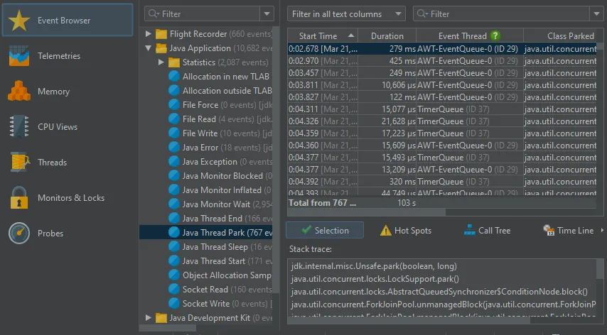
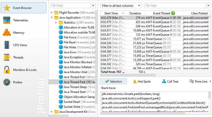
Events are categorized hierarchically and shown in the tree on the left side, single events are displayed in the
table on the right. The columns of the event table and the analysis views below it depend on which event types have been selected.
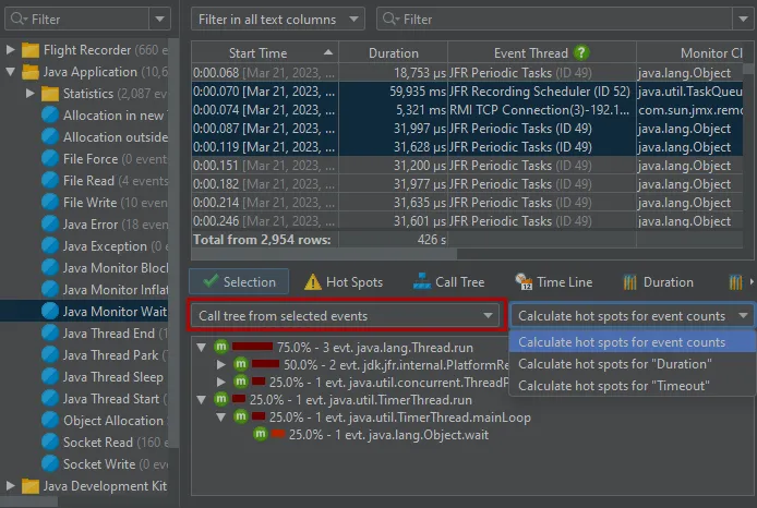
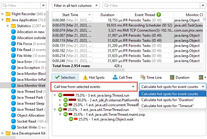
In the selection area, the stack trace of the selected event is shown if it was recorded. If you select multiple events, a call tree or
a hot spots view is shown for them. If the selected event types have time, memory or frequency measurements, you can choose to calculate
the hot spots for any of those measurements.
To avoid overloading the UI, the event table only shows a maximum of 10000 events. The analysis views operate on all events in the snapshot.
Due to the nature of JFR recording, JFR snapshots can become very large, so JProfiler's event browser has been optimized for maximum speed
even for extreme file sizes.
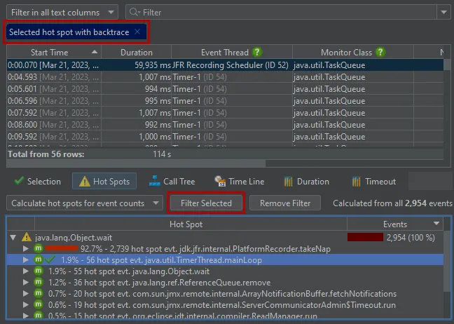
The "Hot Spots" and the "Call Tree" views are like their counterparts in the "Selection" area, but for all events of the selected event
types. Also, you can add call stack filters and hot spot filters and an optional back trace part.
Any analysis view itself is calculated from all filtered events, but excluding the filter that was set in the analysis view itself.
This makes the analysis view more useful because you can see what part of the total event set you have selected there.
The "Time Line" view shows a histogram of all event start times. You can select a time range with the mouse and filter the events
in the table. By default, the view has a logarithmic vertical axis.
For each event column that contains a durations, memory sizes or a frequency, JProfiler adds a histogram view.
Histograms show event counts on their vertical axis while the horizontal axis shows the selected measurement. Bin sizes and event counts
are available from the tooltip. Event filters can be added in histogram views by selecting a range on the horizontal axis.
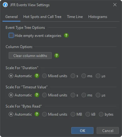
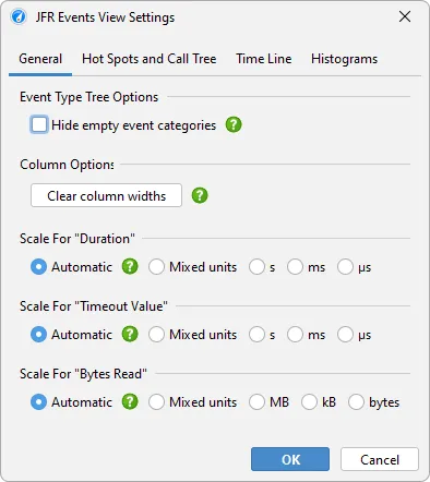
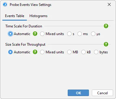
The view settings dialog of the event browser allows you to customize the views. For example, the scales for the columns that are currently
shown can be adjusted there.
Apart from the JFR browser, a subset of JProfiler's views that match with data provided by JFR are available when opening snapshots.
This is a capability that JProfiler already had before. In addition, the new garbage collector probe is now available for JFR snapshots.
Along with the first-class support for opening JFR snapshots, JProfiler adds support for recording JFR snapshots directly
from within JProfiler.
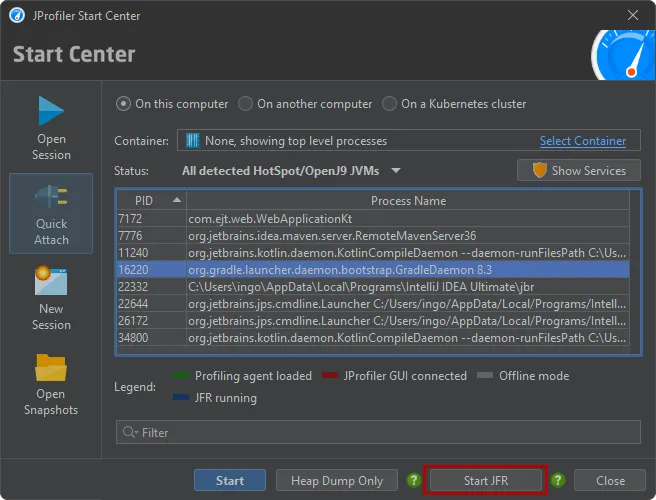
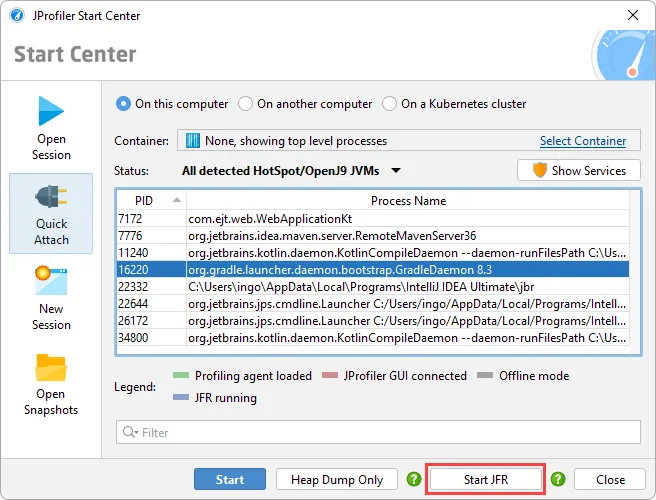
In the attach dialogs where you can attach to a JVM for profiling, you alternatively start JFR recording. This includes all remote
connection capabilities of JProfiler, such as Windows services, SSH connections, Docker containers and Kubernetes.
Even if you are not interested in any particular JFR data, this recording mode can be useful if you are trying to obtain information
about a production environment where a native profiling agent that uses the JVMTI may not be loaded. JFR snapshots can contain
data about the runtime characteristics and even allow you to detect a pronounced CPU hot spot.
This is similar to the adjacent "Heap dump only" option that takes an HPROF memory snapshot without loading the profiling agent.
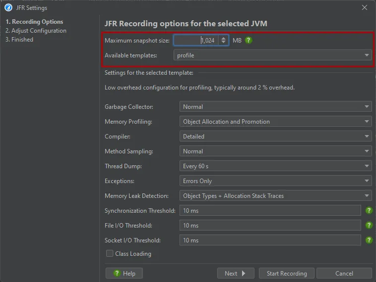
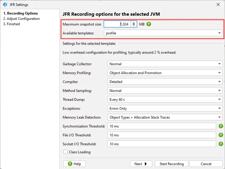
When you start JFR recording, a wizard is shown that lets you choose the JFR recording settings.
To avoid that the JFR recording fills up your entire hard disk, a maximum snapshot size has to be set. If exceeded, old chunks of data are
discarded.
JFR configurations files are located in the "lib/jfr" directory of the JRE. They contain a high-level configuration scheme that is shown as
a UI by JProfiler on the same wizard step.
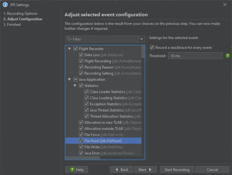
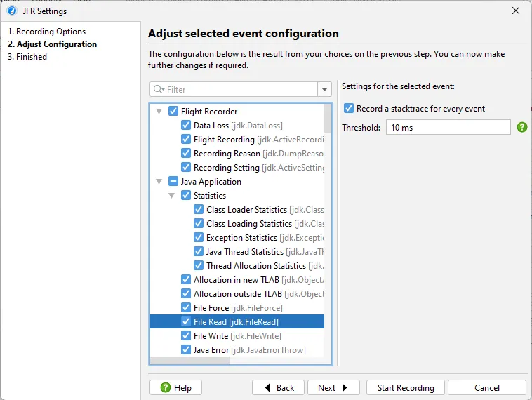
In the next step of the wizard, the result of this configuration is shown as a tree of all JFR events. If you have already profiled this
JRE before, JProfiler will offer you to use the last settings.
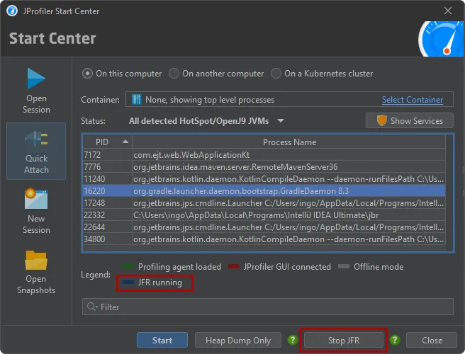
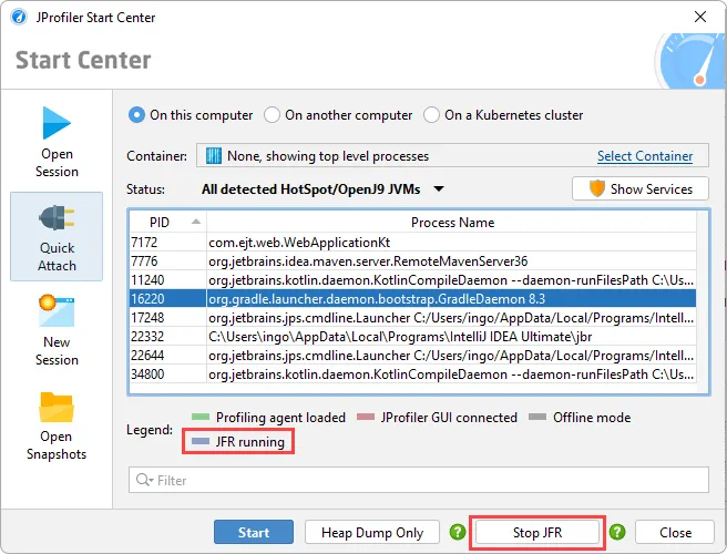
After recording is started, the JFR recording button changes to show "Stop JFR". Also, the background color of the unselected JVM entry in
the table changes to show that a JProfiler JFR recording is running.
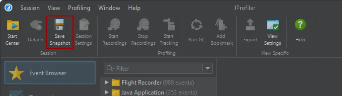
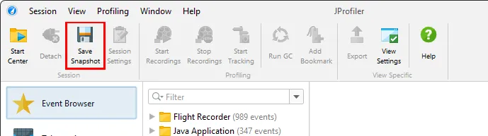
After clicking "Stop JFR", the JFR snapshot is transmitted to the local machine and opened in JProfiler. These snapshots are temporary. If
you want to keep the snapshot for later analysis, you can save them with the "Save snapshot" action.
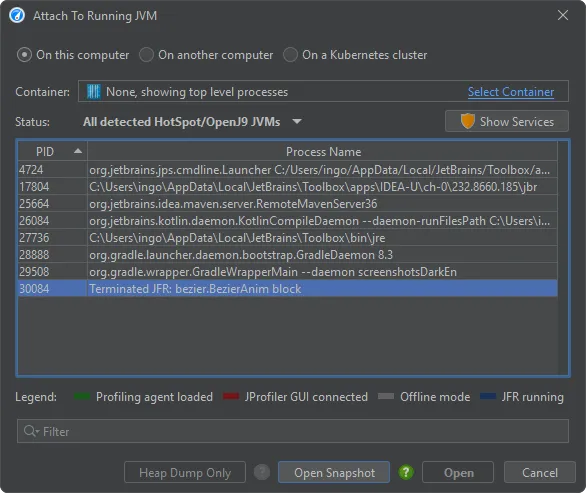
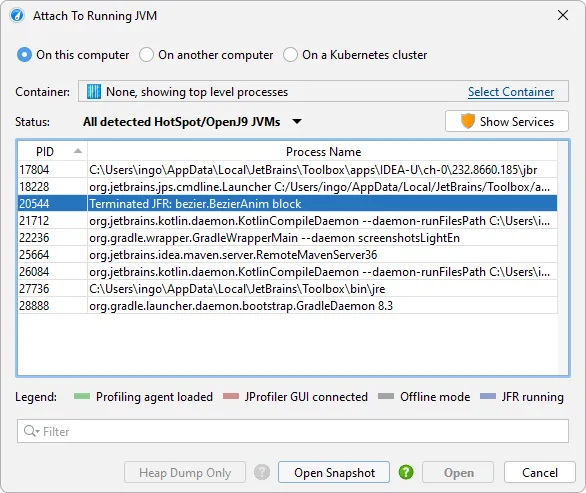
If a JVM where you have started a JFR recording in JProfiler terminates before you open it, the attach dialog will have a "Terminated JFR"
entry for it, and you can use it to download the JFR snapshot that the JVM saved at exit.
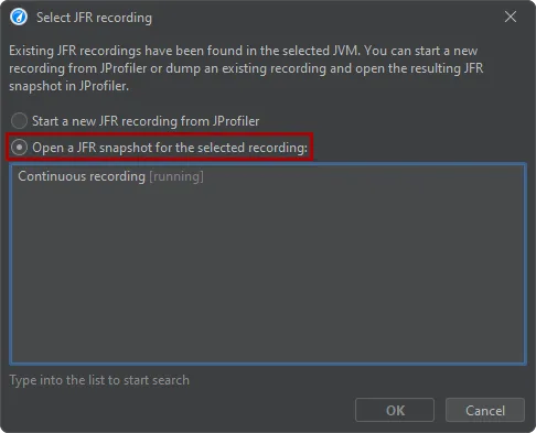
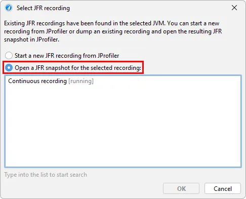
If JFR recordings are running in a JVM that were not started by JProfiler, you can still open them in JProfiler. In that case, JProfiler
will not show the recording wizard when you click the "Start JFR" button but a dialog where you can choose whether to start a new recording
or open an existing JFR recording. Existing recordings will never be stopped by JProfiler.
The probe events view has been improved in many ways. This view is part of nearly all probes.
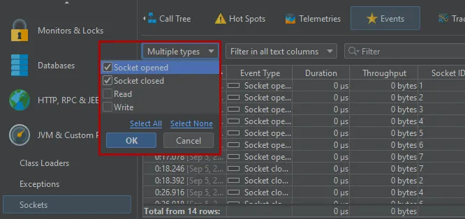
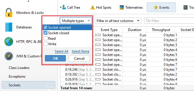
Many probes handle a number of different event types at the same time. The type selector above the events table now allows you to
select multiple event types. For example, in the "Sockets" probe, you can now analyze when sockets were opened and closed without
getting distracted by the intervening "Read" and "Write" events.
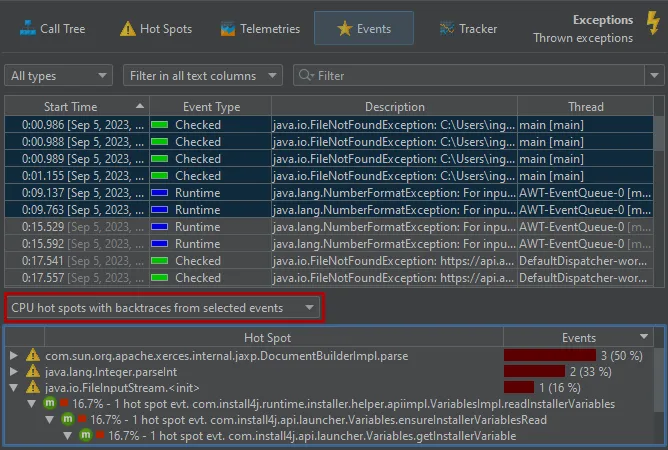
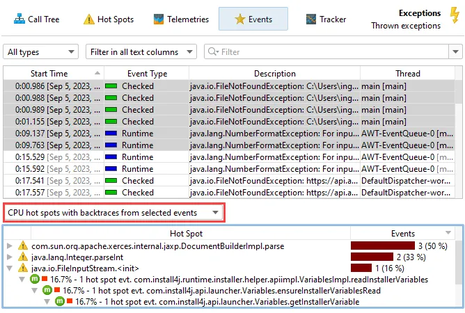
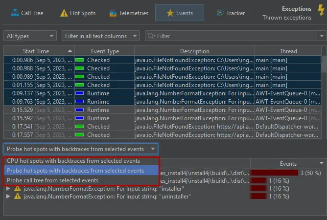
When you select multiple events, the stack trace view at the bottom now shows cumulated data. For example, you can see
the CPU hot spots of the selected events with backtraces.
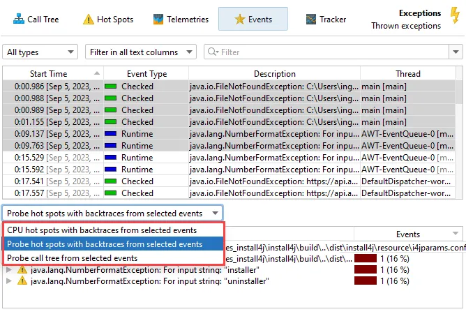
The other available views are the "probe hot spots with backtraces" that have the payload at the top and the "probe call tree".
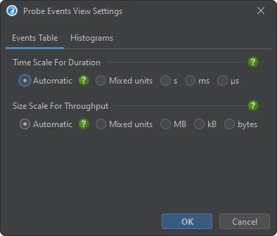
Scales for durations and throughputs can now be adjusted in the view settings dialog of the probe events view and the control objects
view. These settings are saved separately for each probe.
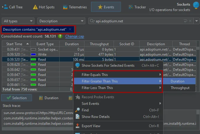
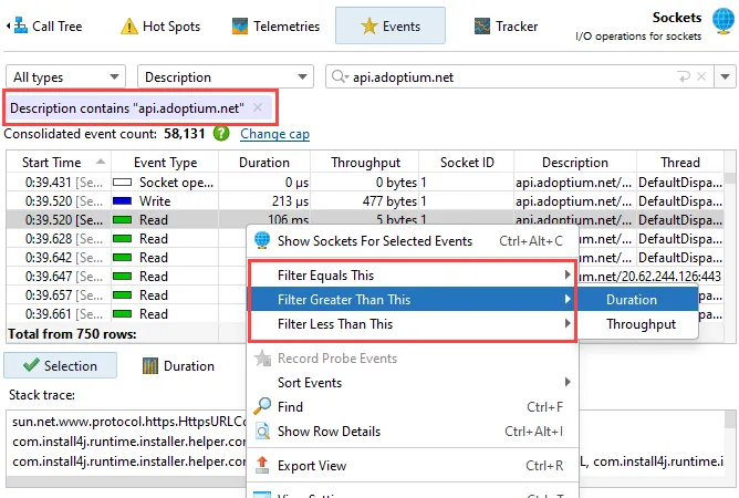
Filtering in the probe events and the control objects views now works on a per-column basis. You can add multiple filters at the same
time, either at the top of the table or most conveniently from the context menu, in order to use a value in the selected row. Filters are
added as tag labels above the table and can be removed individually by closing them.
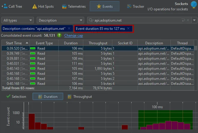
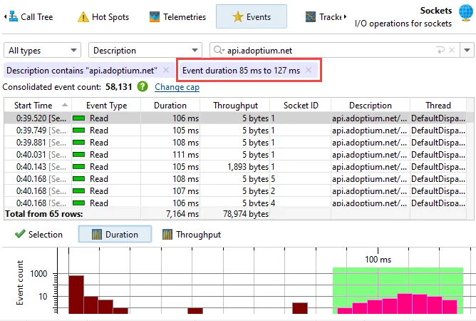
The probe events view now includes a histogram view for event durations and optionally a histogram view for throughputs if
the probe measures memory. By default, the views are logarithmic, so you can easily spot outliers. By selecting a value range on the
horizontal axis, you can add a filter for the probe events table.
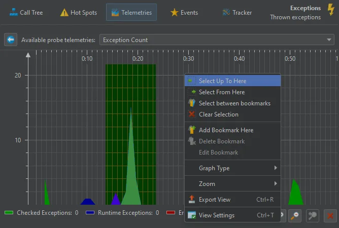
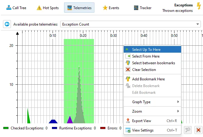
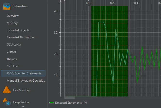
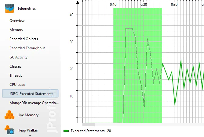
You can now filter probe events by selecting a time range in the probe telemetry views. You can do that either by dragging the mouse
or by using one of the selection actions in the context menu.
Probe event filters can now be set from the probe call tree and the probe hot spots view. The context menu in both tree views
as well as the tool bar has an action to create a filter and switch to the probe events view.
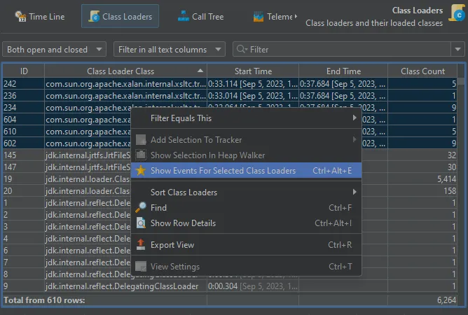
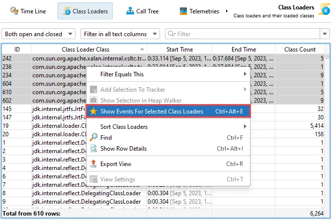
Multiple control objects can now be selected and the associated events can be shown. This allows you to analyze events for an entire
category of control objects.
VM telemetries have been improved.
You can now drag and drop VM telemetries in the overview to change their order. This is useful to compare telemetries of interest. The
change in the order is persistent across profiling sessions and is reflected in the view selector on the left.
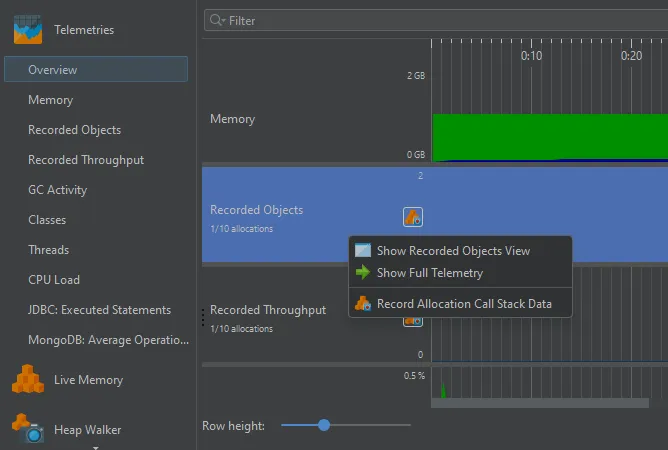
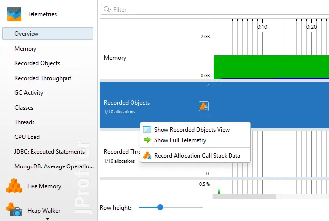
Also, the telemetries from the recorded object views are now always visible, even if no allocations are recorded. In that case, you
will see an inline recording button that lets you conveniently start allocation recording. The context menu also includes the recording action
if you want to stop it again that way as well as other actions to show the recorded objects view or the full telemetry.
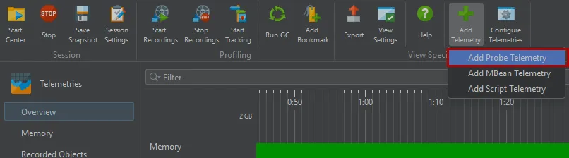
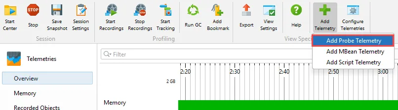
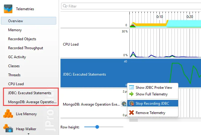
Probe telemetries can be added to the VM telemetries section. Previously, you had to activate a probe and navigate to its telemetry
view to see one of its telemetries. This made it difficult to compare them with the system telemetries or with telemetries from other probes.
Now you can configure a session to include any number of probe telemetries directly in the VM telemetries section.
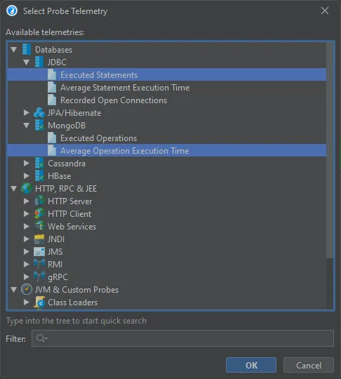
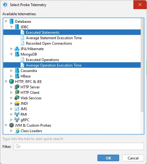
In the probe telemetry registry dialog, all available probe telemetries are listed and you can select multiple telemetries at once.
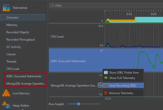
The probe telemetries are added at the bottom, but can be dragged to the desired index in the VM telemetries overview.
Like the telemetries from the recording actions, probe telemetries have an inline recording button if recording is currently stopped, and
the context menu allows you to navigate to the probe view.
In the full probe telemetries, you can select a time range to create a filter in the probe events view, just like in the probe view itself.
After such a selection, the probe events view will be shown.
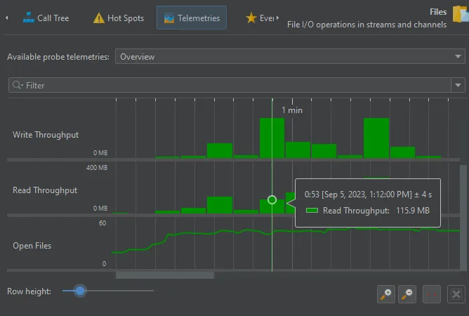
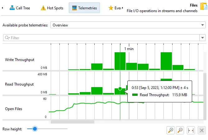
Telemetries that show rates are now shown as histograms. For example, this includes the recorded throughputs in the "Files" probe.
Previously, these telemetries were shown as line graphs which did not give a sense of the total throughputs when looking at time periods
much larger than a minute.
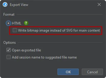
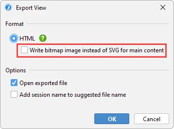
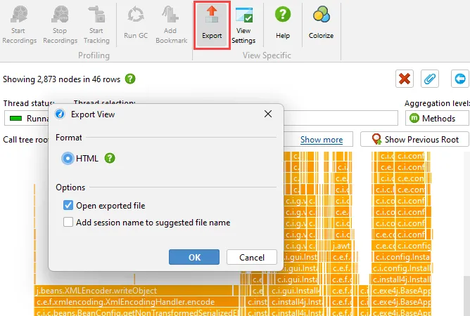
Finally, any telemetry can now be exported as SVG. The bitmap export is optionally still supported.
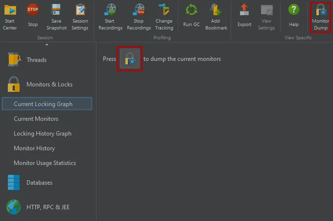
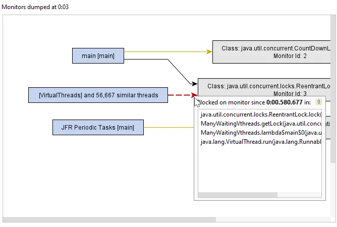
The current locking graph and current monitors views have been improved. These views are principally used for analyzing deadlocks.
Current monitor data is now a snapshot rather than continuously updated. This makes it easier to analyze a single locking situation.
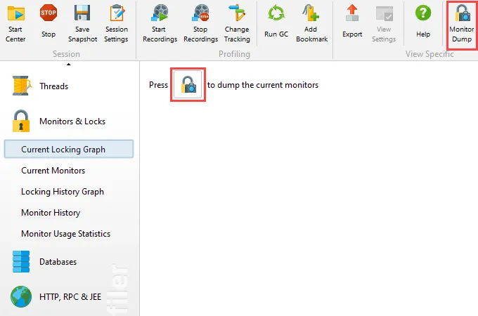
There is an action in the toolbar to dump the current monitors.
The current monitor snapshot also makes it possible to save this information in a JProfiler snapshot or to time the monitor snapshot
programmatically. There is a new method in the controller API as well as a trigger action for this purpose.
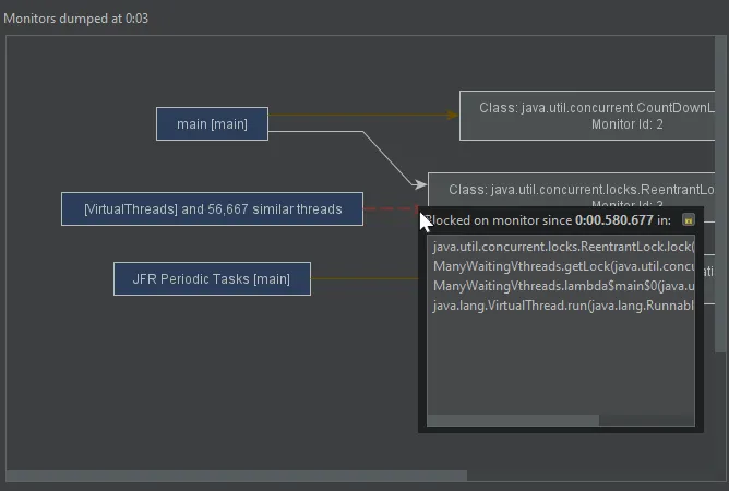
Current monitors and current locking graph views now show java.util.concurrent locks. In attach mode, these views are now
available, but only for java.util.concurrent locks.
Current monitors and locking graph views now group similar threads. This makes it easier to interpret locking situations with many
threads and is important for supporting virtual threads where large numbers of threads may be active at the same time.
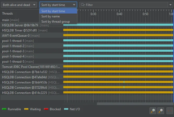
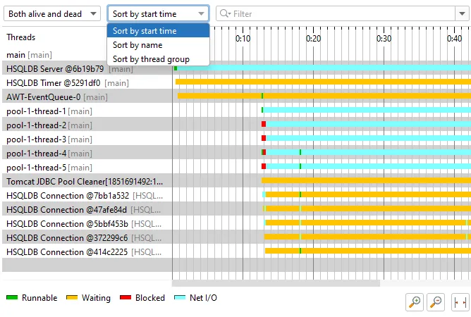
The thread history view and the probe timeline views now support reordering. You can drag threads or control objects to their desired
location or use the sorting drop-down to order the view by start time, by name or by thread group.
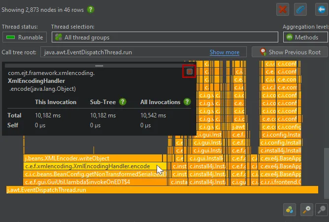
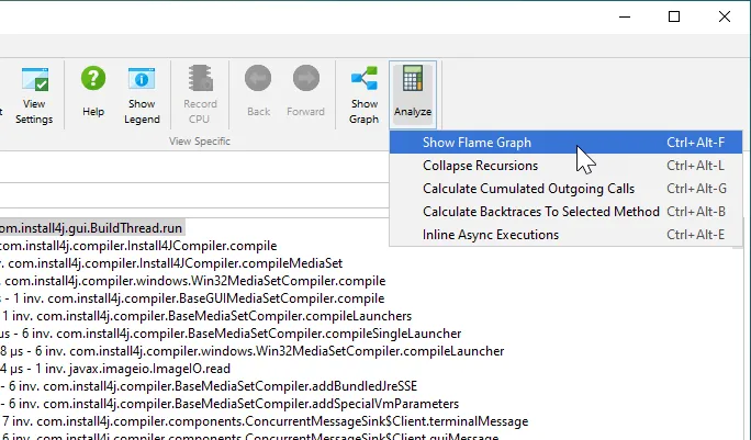
Flame graphs have been improved. Flame graphs are available in call tree views from the "Analyze->Show Call Tree" action.
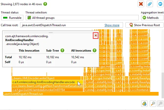
When inspecting the nodes in the flame graph by hovering over them with the mouse, the tooltip can get in the way and obscure part of the flame
graph that you might want to look at. Now you can use the pin button in the top-right corner of the tooltip to move the tooltip to a
fixed location with the gripper at the top. The pin button then becomes a close button.
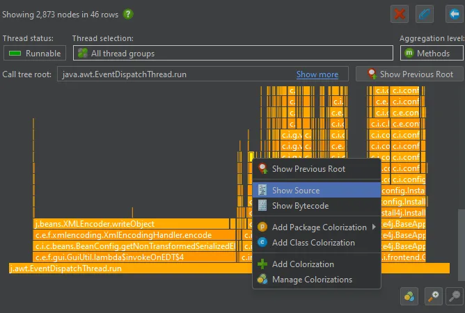
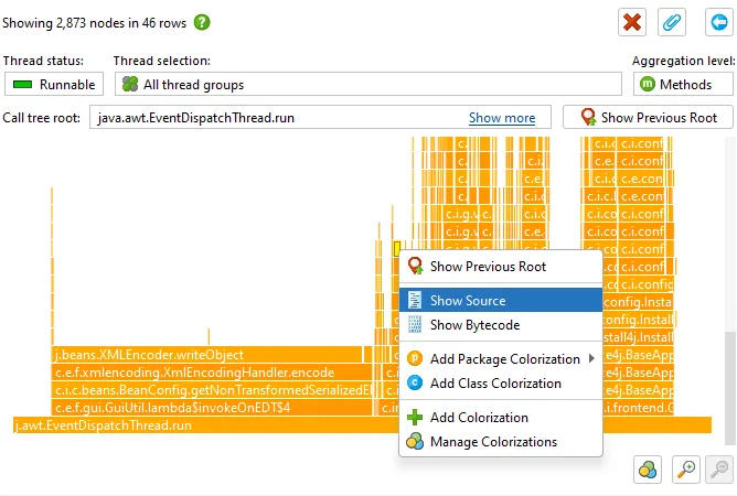
A "Show Source and a "Show Bytecode" action have been added to the context menu in the flame graph. As all such actions in JProfiler,
the "Show Source" action will open the source file in the IDE if you are using an IDE integration.
Flame graph colorizations are now persisted, so you don't have to configure them each time again for new profiling sessions.
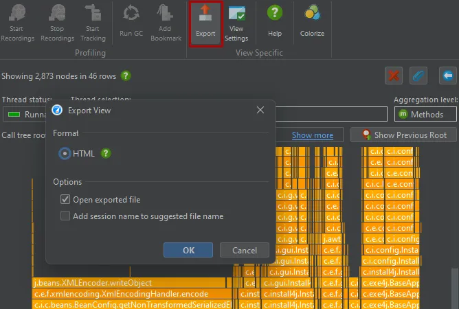
Finally, flame graphs can now be exported as SVG. The exported SVG has basic tooltips so you can see the method names and their times.
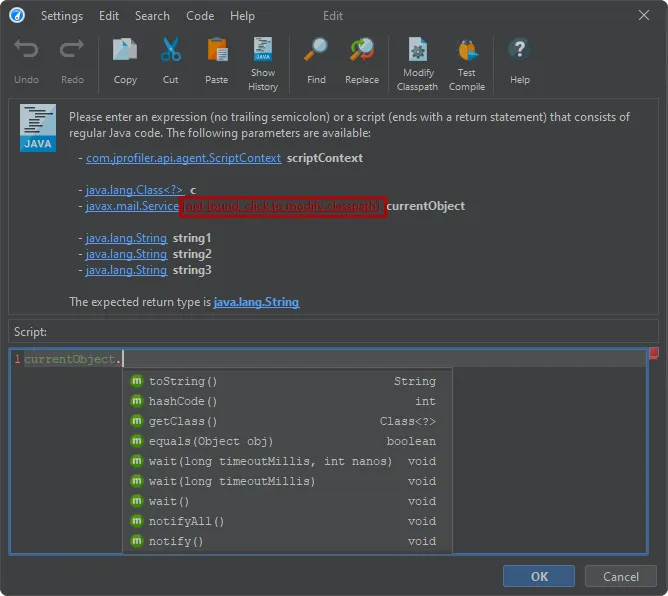
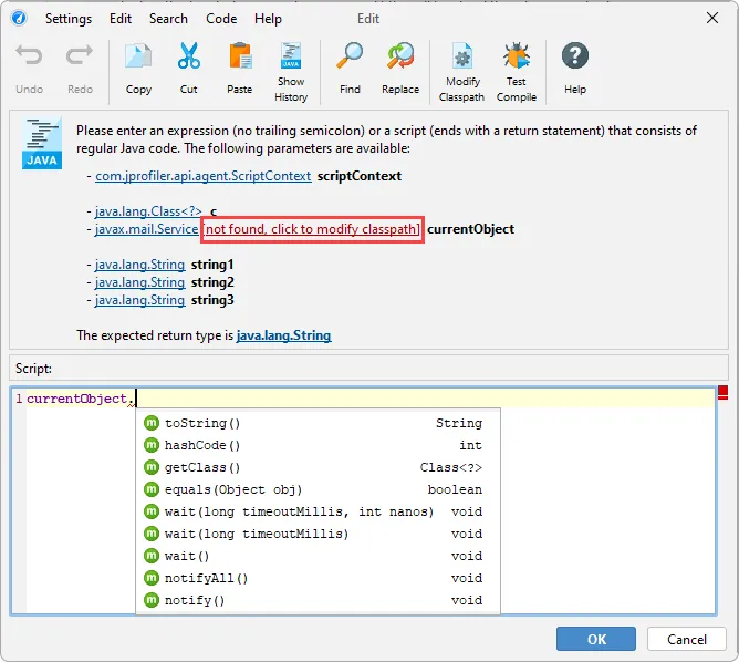
An action to modify the session classpath has been added to all script editors. Many features in JProfiler allow you to enter a
script for various purposes. For example, the "Split method with a script" action is available in the context menu of the call tree view.
If the class of the method or a class of a parameter is not in the configured session classpath, JProfiler cannot provide code completion
or compile a script that uses its members.
To solve this problem conveniently, JProfiler now adds action labels to modify the session classpath right next to the missing classes in the
script header. After adding the relevant JAR files to the classpath, you will be able to use the classes in the script immediately.
Attach mode was improved.
In the list of attachable JVMs, JProfiler now shows the JRE path when no other naming information about the application is available.
Because many applications use a private JRE, this makes it possible to identify those applications.
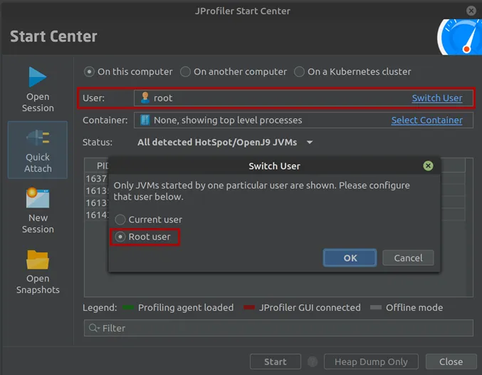
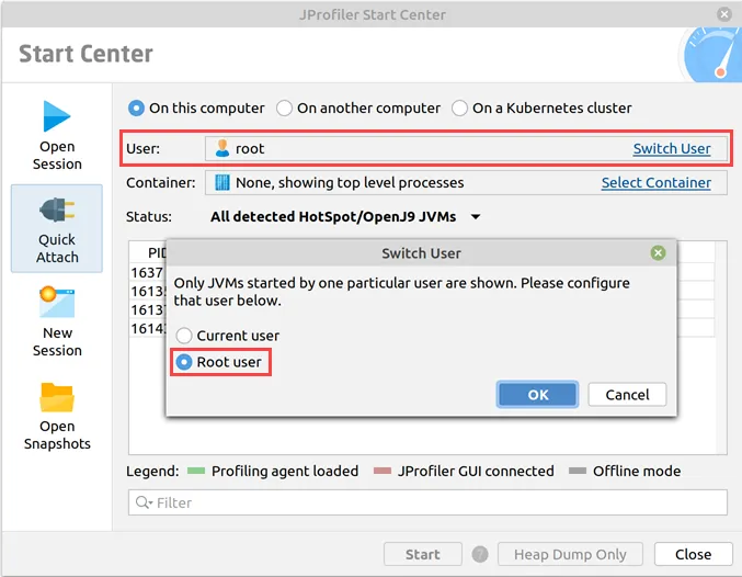
On Linux, you can now attach to processes that were started by systemd with "PrivateTmp=yes" in the systemd unit file. You have to use
the root user to attach to such processes.
Also on Linux, JProfiler now inspects the mounts that were namespaced per-process to find writable directories. This affects daemons launched
by systemd with "ProtectSystem=strict" in their system unit file, for example.
Added support for Linux Alpine ARM.
JVMs on this architecture can now be profiled by JProfiler.
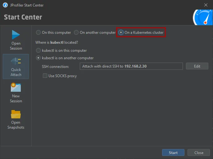
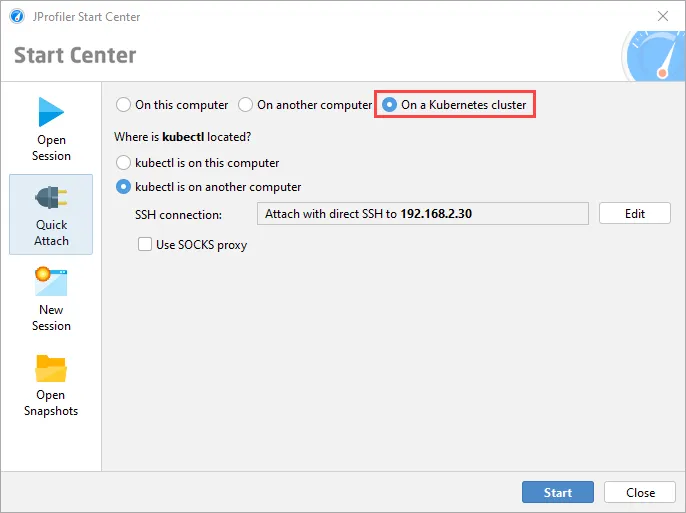
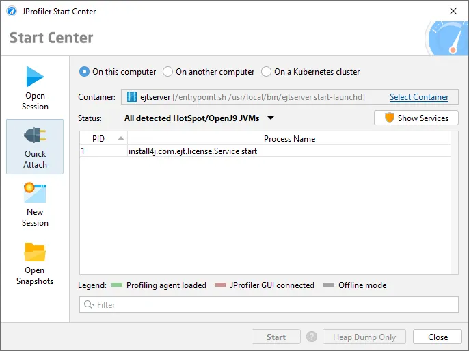
Support for attaching to JVMs running in a Kubernetes cluster has been added. The attach window now offers three main modes: Besides
the existing radio buttons for JVMs running on the local machine and a remote machine there is now a Kubernetes cluster option.
JProfiler uses the "kubectl" command line utility which can be available locally or on a remote machine via SSH.
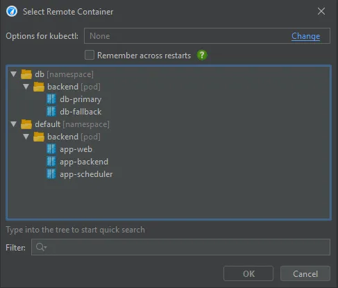
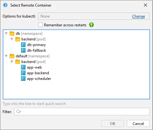
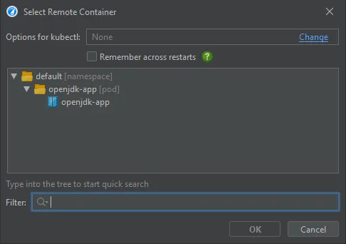
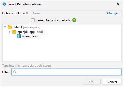
After clicking on "Start", you can select a container in a tree of Kubernetes namespaces and pods.
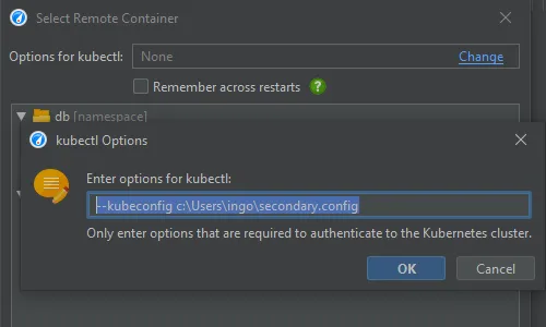
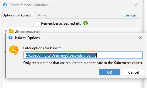
JProfiler assumes that kubectl is already configured to connect to your cluster. If special command line options are required, they can be
configured at the top of the dialog and can be made persistent on request.
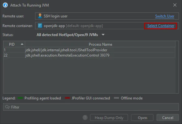
After selecting the container, you can select from all JVMs that are running in the container. Should you need to switch to another container
in your Kubernetes cluster, you can do so with the "Select Container" action.
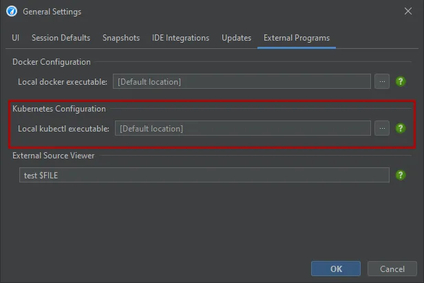
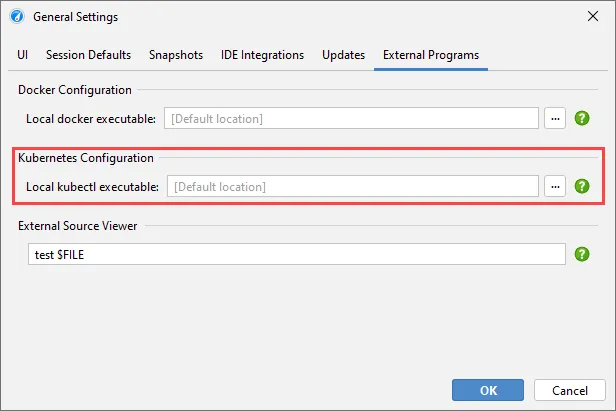
If you choose to execute kubectl locally, the location of kubectl is detected automatically and can be adjusted in the general settings if
required.
JProfiler can now attach to JVMs running in Docker Desktop on Windows and macOS and on local Docker installations on Linux.
Previously, only Docker on remote Linux hosts was supported.
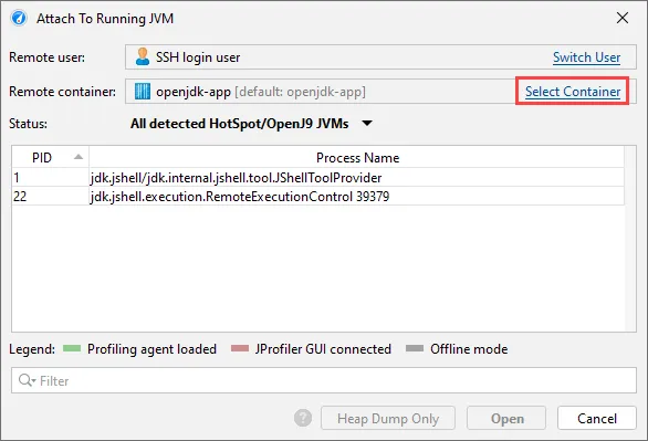
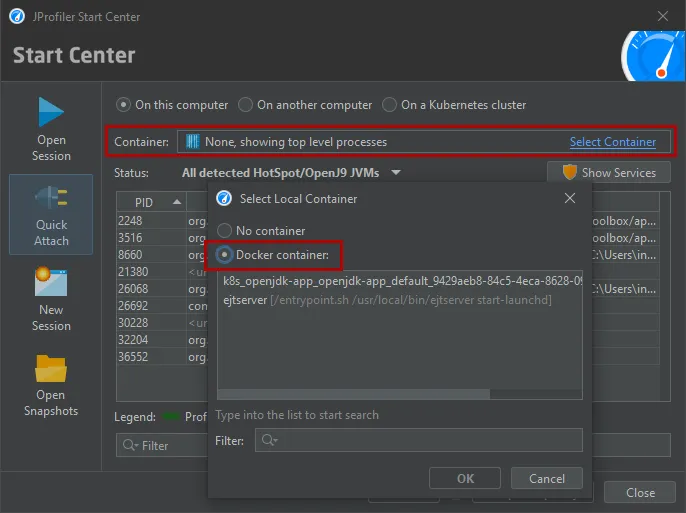
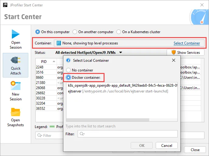
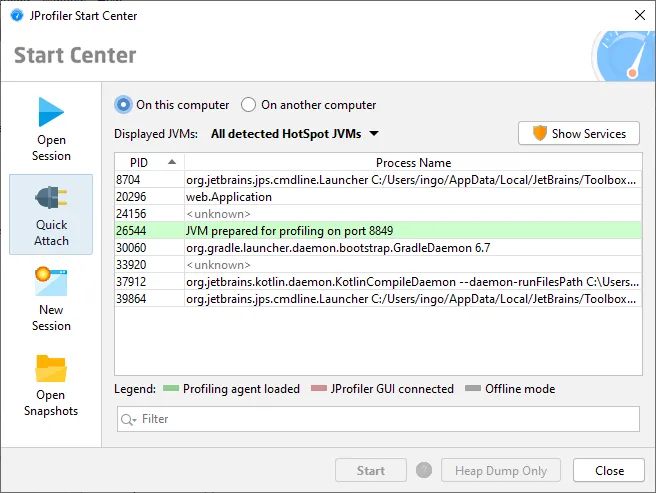
To attach to a Docker container that is running locally, go to the "Quick attach" dialog, select the "On this computer" section and click on the
"Select Container" link.
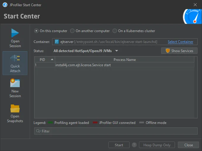
After selecting the container, the list of JVMs that are running in the container will be shown and you can proceed just like when attaching
to a JVM that is running directly on the local machine.
As shown above, the selection dialog may contain locally running Kubernetes containers. You can also use the Kubernetes attach
instead of the Docker attach in this case. Instead of generated names starting with "k8s", the local Kubernetes attach will show
more informative container names.
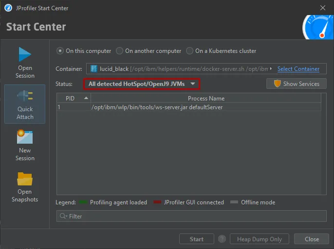
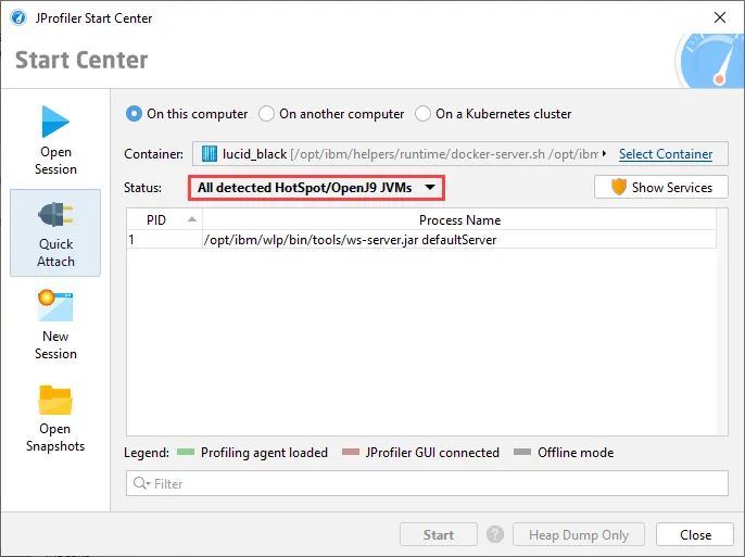
Support for attaching to OpenJ9 JVMs has been added. It requires a recent OpenJ9 JVM (8u281+, 11.0.11+ or Java 17+) or an IBM
JVM that is based on such a release.
Previously, the only way to profile OpenJ9 and IBM JVMs was to add the -agentpath VM parameter at startup.
This is especially important for profiling OpenJ9 and IBM JVMs running in containers where attach mode is the only way to profile without
undesirable modifications of the container. For example, you can now attach to the Websphere Liberty
Docker container without any further configuration.
Attach functionality has been improved in several ways:
- A user switcher has been added on Linux to profile JVMs started by different users
- Support has been added for attaching to JVMs running in Redhat UBI-minimal images
- FreeBSD and AIX are now supported target platforms for the remote attach functionality
- On Windows it is now possible to attach to a JVM started by the same user but running in a different session
- Elevated users can now attach to JVMs started by any user with jpenable on Windows when the PID is provided as long as the JProfiler installation is readable for that user
- Different temporary directory settings for JProfiler and the profiled JVM no longer prevent attaching on Windows when a PID is provided for jpenable
OpenWebStart can now be profiled by JProfiler. After the discontinuation of Java Web Start in Java 11,
OpenWebStart has been developed as a drop-in open source reimplementation based on IcedTea-Web
by RedHat.
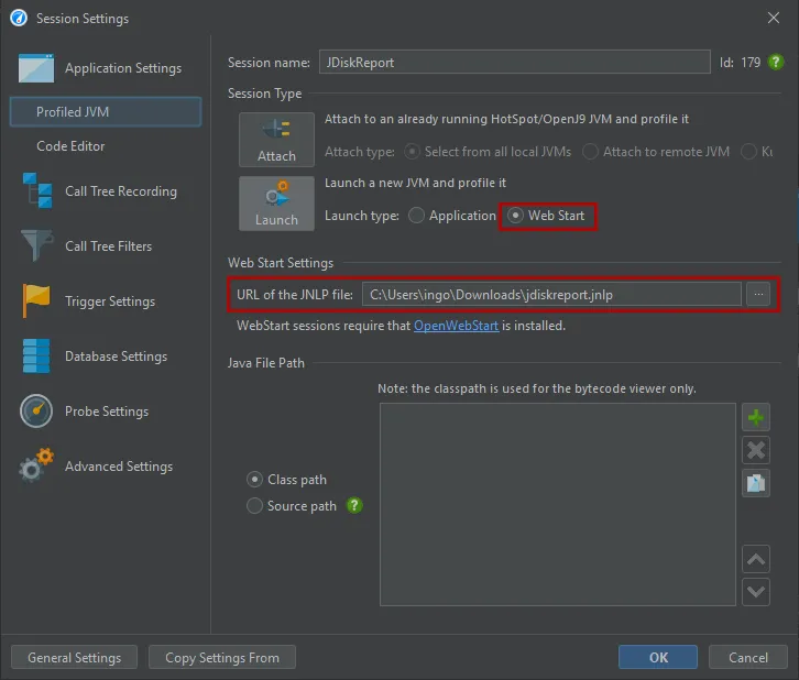
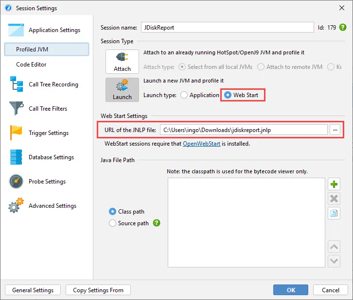
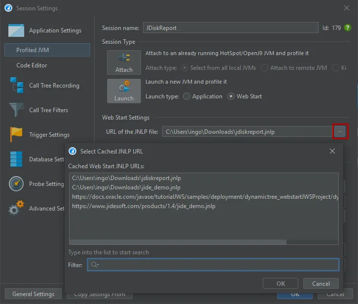
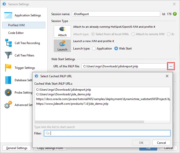
JProfiler now offers a Web Start session type where the only thing that you have to configure is the JNLP URL in order to start profiling.
All JNLP URLs that have already been executed by OpenWebStart are shown in the chooser dialog.
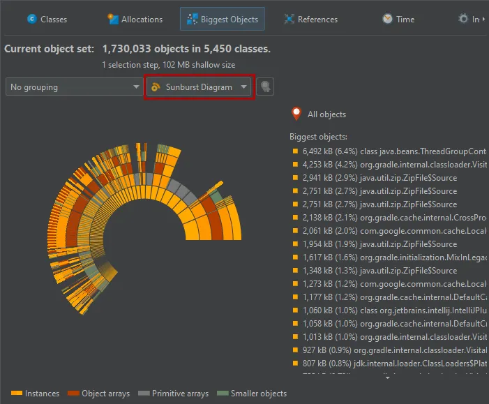
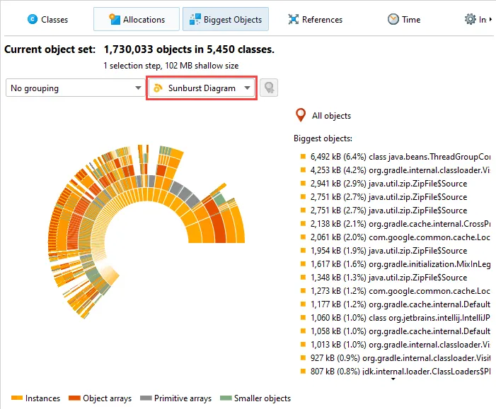
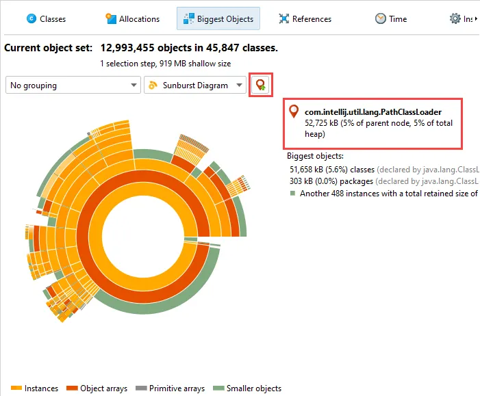
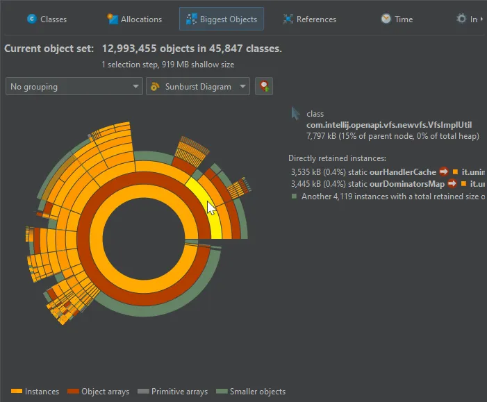
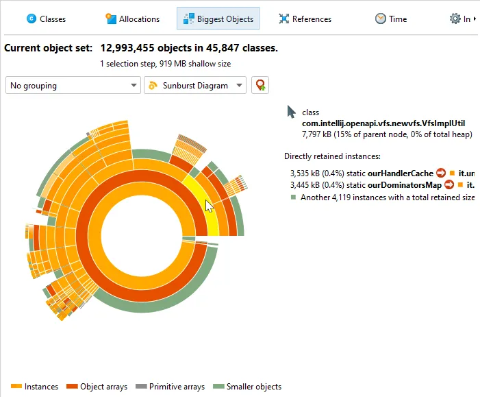
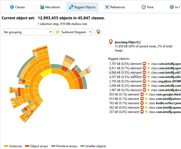
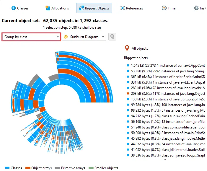
A sunburst diagram visualization has been added to the biggest objects view of the heap walker. By default,
the biggest objects view continues to show the tree view, but you can change the display with the view mode chooser at the top.
The diagram is composed of a series of concentric segmented rings and shows the entire content of the dominator tree up to
a maximum depth in one single image. References originate in the innermost ring and propagate towards the outer
rim of the circle.
This visualization gives you a flattened perspective with high information density that allows
you to discover reference patterns and see large primitive and object arrays at a glance through their special
color coding.
Clicking on any ring segment sets a new root for the circle, thereby expanding the maximum depth that you can
see in the diagram. Clicking on the hollow center of the diagram restores the previous root.
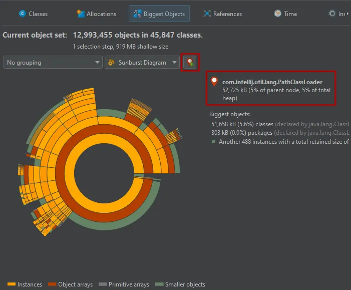
More information about instances and their immediately retained objects is displayed on the right side of the
diagram when you hover over them with the mouse. When the mouse is outside any ring segment, the list on the
right side shows the biggest objects in the innermost ring.
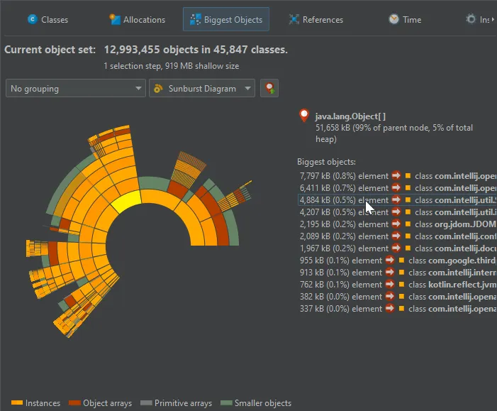
Hovering over the list of biggest objects on the right highlights the corresponding ring segments and clicking on a list item sets
a new root for the diagram. To create a new object set, you can choose from the actions in the context menu, both on the ring segments
as well as on the list items.
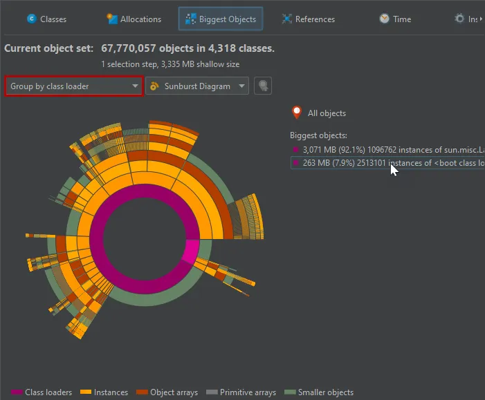
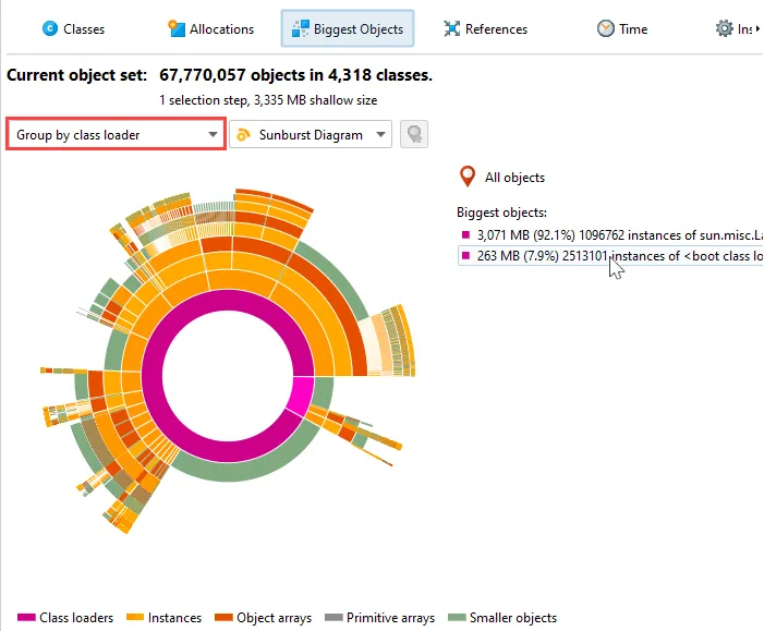
As for the tree view mode, you can group the analysis by class loaders. The class loaders will be shown in the innermost ring.
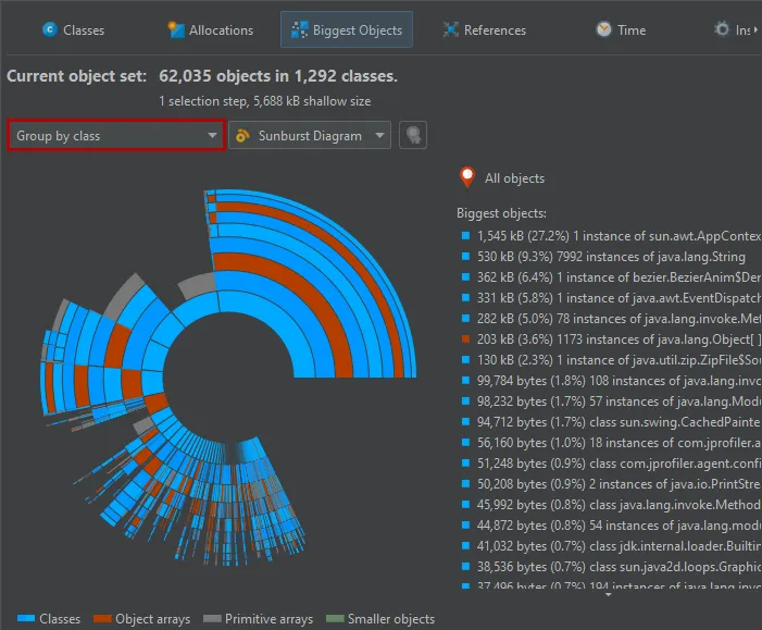
An additional grouping mode that can also be combined with class loader grouping is grouping by classes. If selected,
all biggest objects of a particular class at the same reference level are combined into a single node.
The Reactor Netty web client is now supported for the HTTP client probe.
This goes together with support for the Spring WebFlux HTTP client that uses Reactor Netty under the hood by default.
The Spring WebFlux HTTP client is also supported with the Apache HTTP client.
In addition to the HTTP client probe, the support for the Reactor Netty and Spring WebFlux HTTP clients is important for HTTP tracking
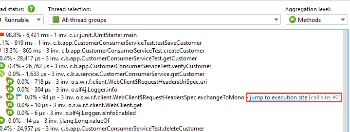
where HTTP call sites are annotated with hyperlinks in the call tree view.
If the server JVM is profiled at the same time in a different JProfiler window, clicking on the hyperlink will show the execution site in that window.
Remote request tracking not only works with live sessions, but also with snapshots.
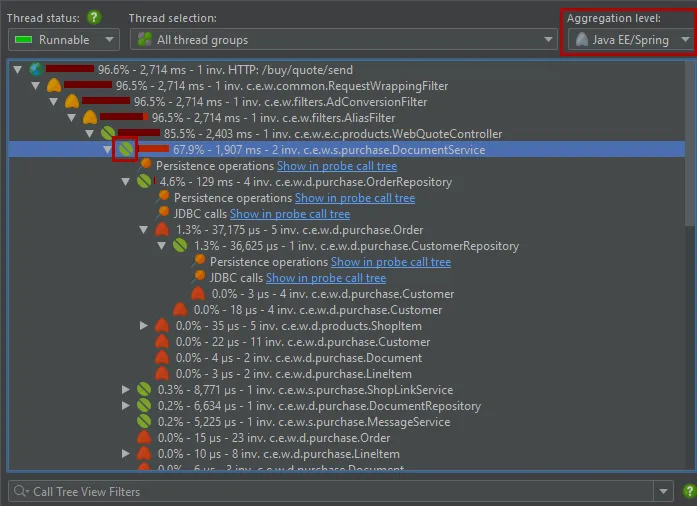
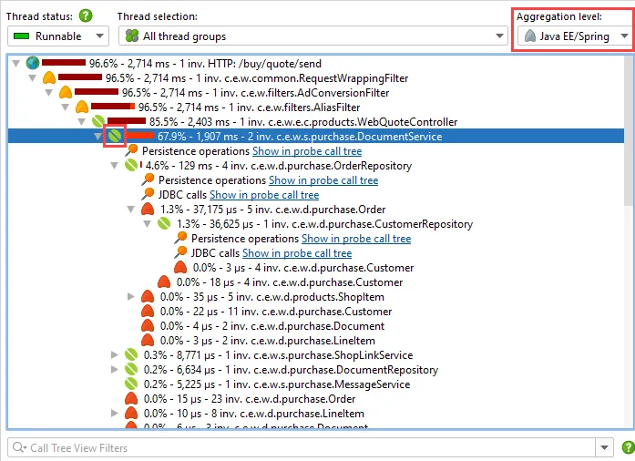
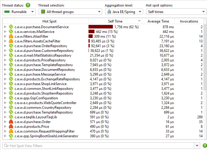
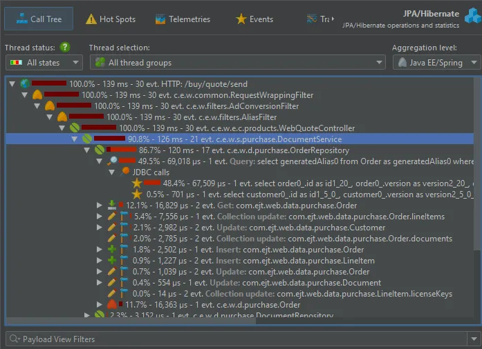
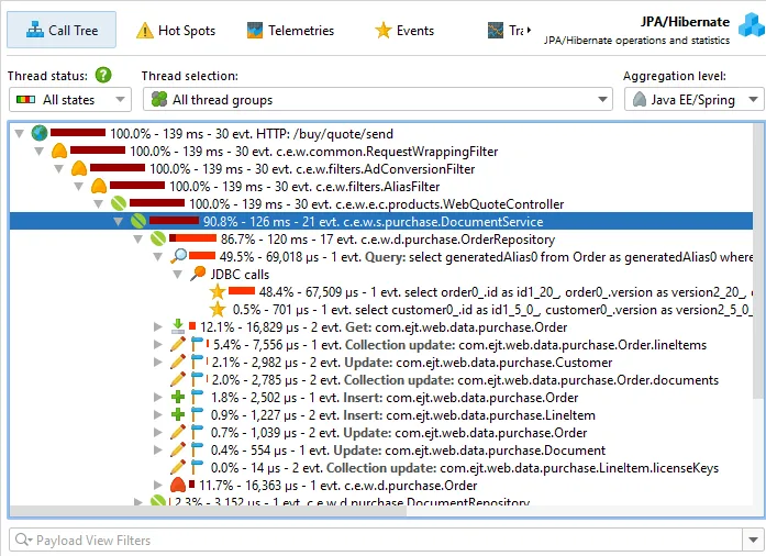
The JEE/Spring aggregation level provides a high-level view for the call tree where only Spring beans and JEE components like
servlets or EJBs are shown. All classes that have been annotated by @Component or any derived annotation like @Service
or @Repository are detected as Spring beans.
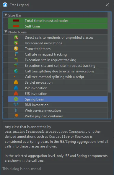
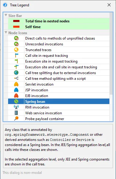
JEE and Spring bean nodes are explained in the tree legend dialog that is available from the tool bar in all views that show a call tree.
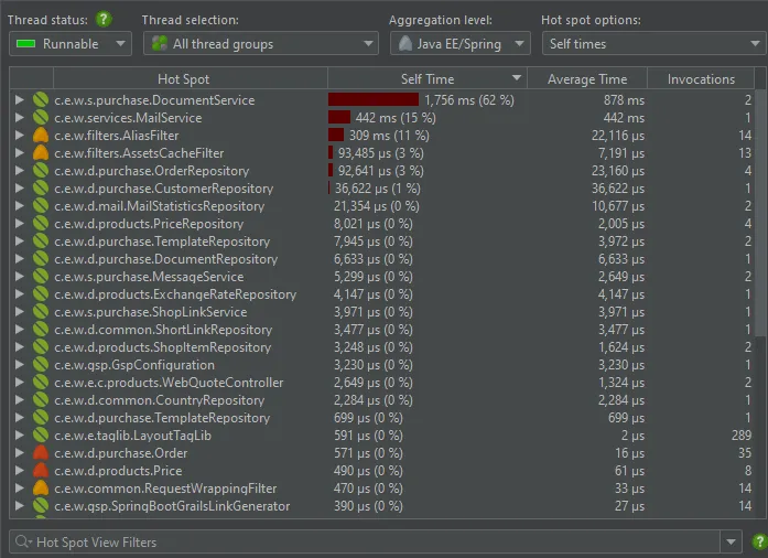
This aggregation level is especially useful for the hotspots view, where it shows hot spots that are determined not on a per-method basis
but on a per-bean basis. All details of the operations that are performed in other classes and library calls are included in the Spring bean
nodes.
Aggregation levels can not only be selected in call tree views, but also in allocation and probe views.
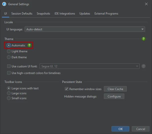
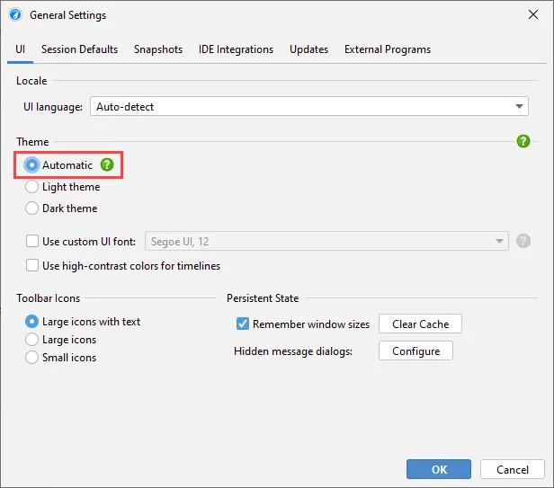
JProfiler now supports live switching between light and dark mode. When the OS theme changes, JProfiler will switch automatically.
In the general settings, it is also possible to select a fixed theme.
Probes in JProfiler now support the following recent releases:
- Hibernate 6
- RestEasy 6
- Ktor 2
- MariaDB connector 3
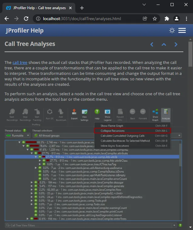
The documentation is now available in dark mode. The default theme follows the OS theme and can be switched manually in the top right
corner.
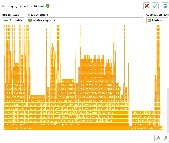
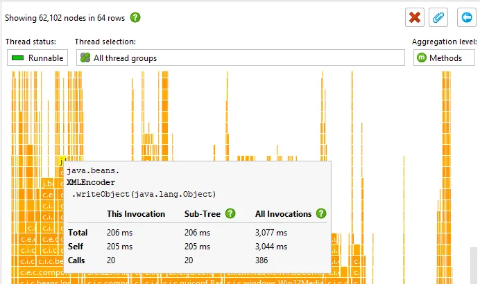
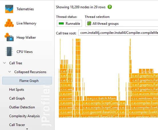
Flame graphs have been added. All views that show call trees can alternatively be shown as flame graphs
that show the entire content of a call tree in one image. Calls originate at the bottom of the
flame graph and propagate towards the top.
Flame graphs are implemented as a call tree analysis and are nested below the current call tree view.
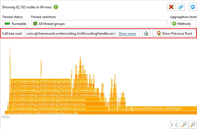
By selecting a node in the call tree, you can set the initial root node for the flame graph.
Child nodes are sorted alphabetically and are centered on their parent node. Due to the self-time that is
spent in each node, the "flames" get progressively more narrow toward the top. More information about nodes
is displayed in the tool tip.
Flame graphs have a very high information density. You can zoom in on areas of interest, or set a new root
node by double-clicking on it. When changing roots multiple times in a row, you can move back again in the
history of roots.
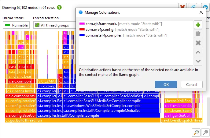
Another way to analyze flame graphs is to add colorizations based on class names, package names or arbitrary
search terms. The first matching colorization is used for each node.
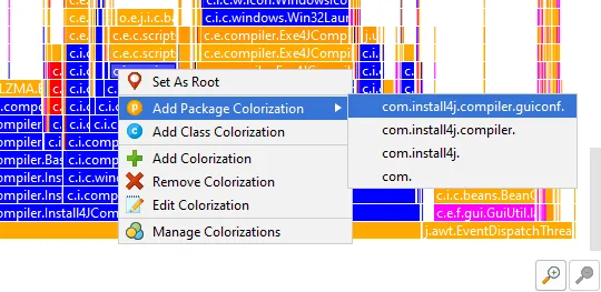
Colorizations can be conveniently added and removed from the context menu.
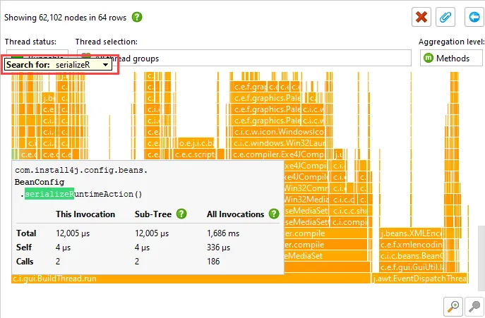
In addition to colorizations, you can use the quick search functionality to find nodes of interest. With the
cursor keys you can cycle through match results while the tooltip is being displayed for the currently
highlighted match.
Flame graphs are not only available for top-level call tree views but also for the results of other call
tree analyses, such as "Collapsed recursions".
Support for Netty has been added. The previous "Servlet" probe and the Netty functionality were merged
into the new "HTTP Server" probe.
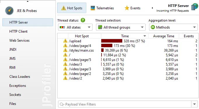
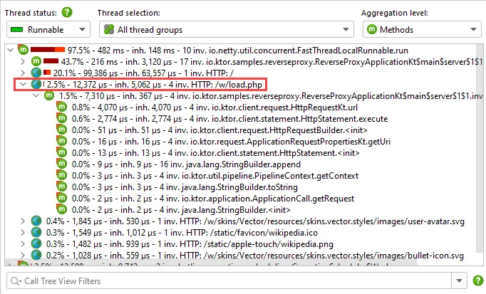
If you are running a Netty-based web server like Spring Reactor,
Vertx or Ktor, the HTTP Server probe shows you the intercepted URLs with invocation counts and well as their
total and average processing times.
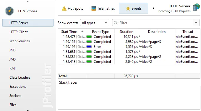
The events view of the HTTP Server probe can list the single URL interceptions chronologically.
Just like for Servlet containers, the call tree is split for each URL, so you can see associated subtree
separately.
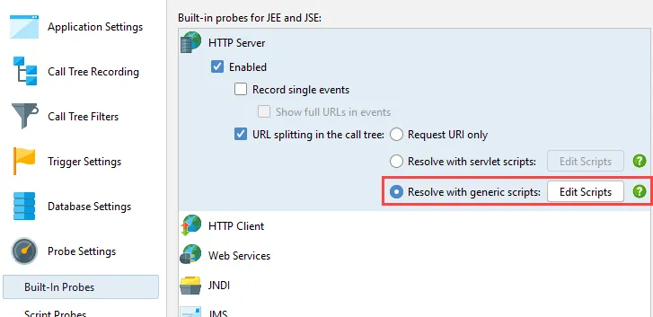
To determine the granularity of the split as well as the displayed URL, the probe settings of the HTTP server
probe now offer generic splitting scripts in addition to the Servlet scripts.
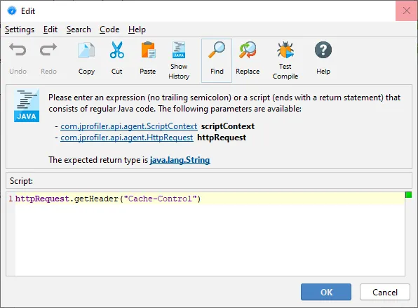
Unlike for Servlet scripts that offer the HttpRequest object from the Servlet API as a parameter, the Netty
landscape is less stable with several incompatible APIs. This is why JProfiler offers an HttpRequest parameter
from its own API to provide access to common request properties. Advanced use
cases can get the underlying Netty request object via the getRequestObject() method.
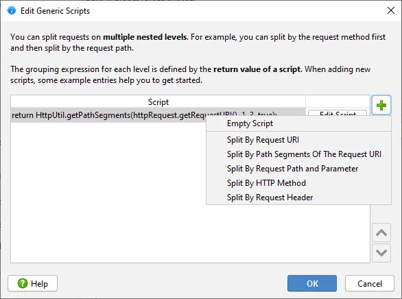
As with Servlet scripts, you can configure a list of scripts to create multiple nested splitting levels in the
call tree. Several script templates for common tasks are available.
Netty is mostly used for async handling of HTTP requests. Because of the associated thread changes, the
subtree below an URL in the call tree will not show the entire handling of the request.
With the async request tracking functionality in JProfiler, you can follow the entire execution flow.
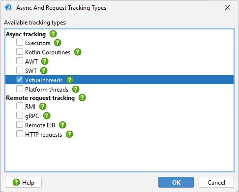
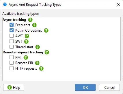
Most frameworks, like Spring Reactor use executors for async handling, so the "Executors" request tracking
type has to be activated. If you are using a server based on Kotlin Coroutines like Ktor, then "Kotlin Coroutines"
is the required tracking type.
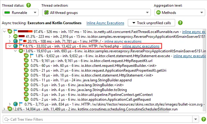
If async tracking is used, the call tree view will suggest to inline async executions both on top of the view
as well as on the call sites where the async calls are initiated.
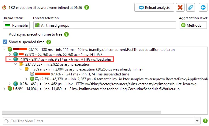
The result of the "Inline async executions" analysis then contains a single call tree across all
involved threads that show you the entire handling of a particular request URL, cumulated for all
matching requests.
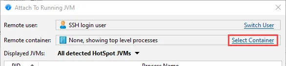
Attaching to JVMs running in Docker containers is now supported in the SSH remote attach
functionality.
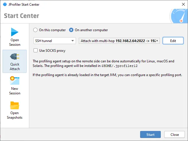
You start out by using the quick attach functionality with an SSH tunnel to a remote Linux machine.
Initially, the JVM processes running directly on the remote machine are listed.
At the top of the remote attach dialog is a line that shows the currently selected remote Docker container.
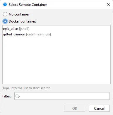
With the Switch container hyperlink you can then choose a running Docker container.
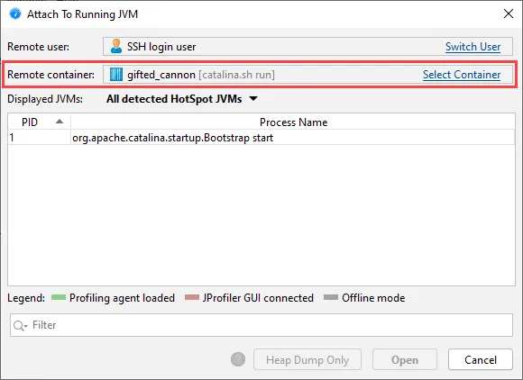
After selecting a Docker container, all JVMs that are running in it are shown. JProfiler will then use Docker
commands to automatically install the profiling agent in the selected container, prepare the JVM for profiling
and tunnel the profiling protocol to the outside.
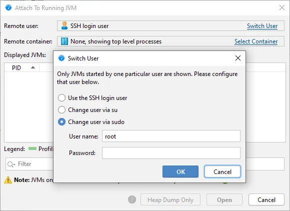
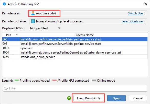
If the SSH login user is not in the docker group, you can switch the remote user first.
Attach functionality has been improved in several ways.
JVMs that have been started with the "-agentpath" VM parameter for profiling are now shown in the attach dialog,
both for local and remote attach. These JVMs are waiting at startup for a connection from the JProfiler GUI.
In that state, the normal attach mechanism in the JVM is not yet available, so an alternative attach mechanism
had to be implemented.
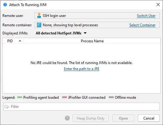
Previously, when connecting to a remote machine, a JRE had to be available for the login user, or the connection
would fail. Starting with this release, a message is shown in the JVM list with a hyperlink to manually enter
a path to a JRE. This allows you to switch to a user that may have access to a JRE or switch to a Docker
container that contains a JRE.
Previously, when changing the user on the remote machine, no HPROF snapshots could be taken.
In this release, a method to transfer the heap dump data between accounts has been implemented and the
"Heap dump only" action is now enabled.
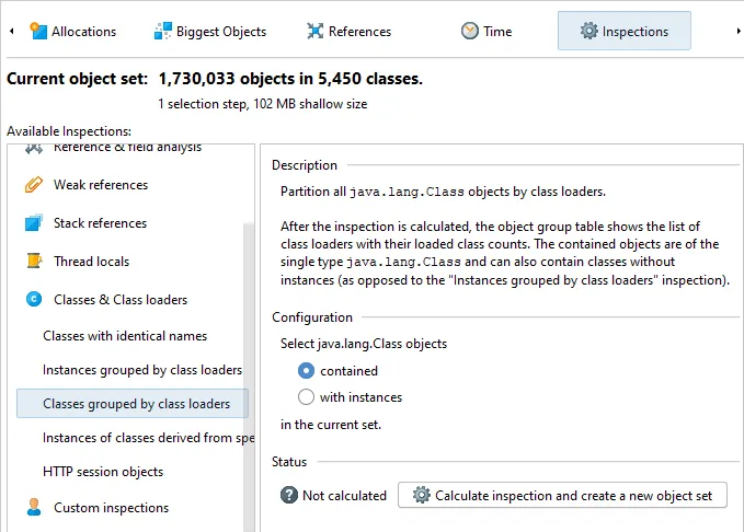
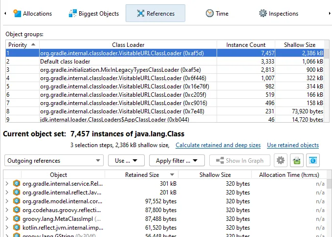
An inspection to group classes by their class loader has been added to the heap walker. This inspection
groups java.lang.Class objects and is complementary to the existing inspection that can group instances
by their class loader.
The result of the inspection can either include classes whose java.lang.Class objects are contained
in the current object set or classes that have instances in the current object set.
When you select a class loader in the grouping table at the top, the corresponding java.lang.Class
objects are shown in in the data views below.
Jakarta EE 9 is now supported. Jakarta EE 9 switches the packages for the API from javax.*
to jakarta.*. JProfiler now supports both the old as well as the new packages for the "HTTP server"
probe.
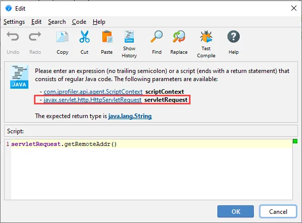
When writing URL splitting scripts in the JProfiler UI, a javax.servlet.http.HttpServletRequest request
object is available as a parameter. If the profiled container supports Jakarta EE 9, calls into the servlet API
are transparently translated into the jakarta.servlet. namespace.
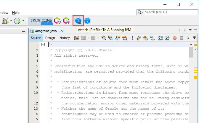
The NetBeans plugin has been improved. An action has been added to attach to a running JVM.
This is especially important for profiling Maven projects that do not use the exec plugin as well as Gradle
projects where the JProfiler plugin has no way to insert VM parameters into the Java invocation.
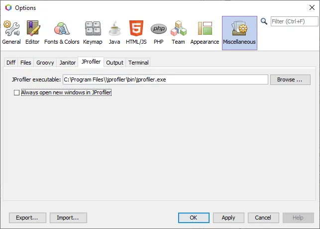
A preference page has been added where you can adjust the JProfiler executable as well as the window policy
for opening new profiling sessions. All other settings continue to be available the session startup dialog
and are saved separately for each NetBeans project.
JProfiler has a new cross-platform light mode. This the new light look and feel
from the IntelliJ IDEA platform.
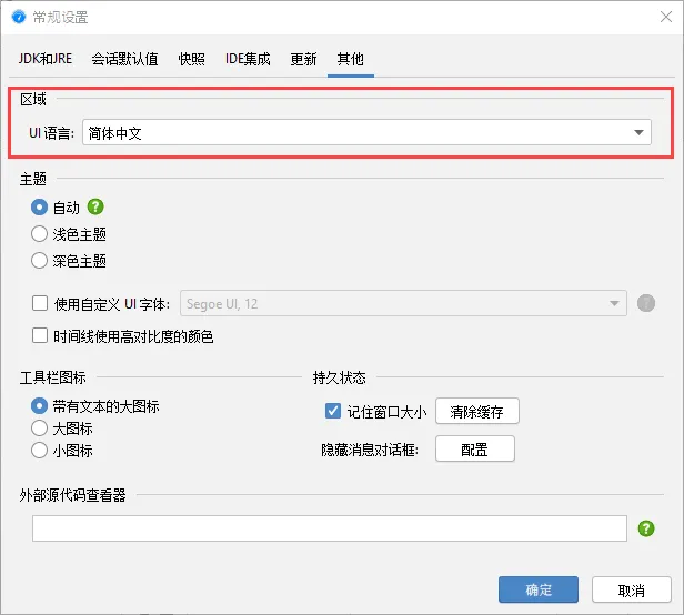
A localization into simplified Chinese has been added. If the locale of your machine is "zh_CN", the
installer will pick it up automatically, otherwise you can switch languages in the general settings dialog.
Support for profiling on Alpine Linux has been added. Alpine Linux is especially popular for Docker
because of its smaller image size. It uses a different C standard library than other Linux distributions,
so the native profiling agent needs a separate port.
Starting with this release, the musl-x64 architecture is included in JProfiler.
Support for profiling on macOS ARM has been added. While profiling JVMs compiled for the x86
architecture is possible on new ARM-based macOS machines via Rosetta, new JVMs compiled directly for the new
ARM architecture require a different native profiling agent.
Starting with this release, the macOS profiling agent is a universal binary that contains implementations for
both x64 and ARM64.
At the time of the 12.0 release, JProfiler is not bundled with an ARM JRE yet, so the JProfiler GUI will run
via Rosetta on macOS ARM machines. A release that includes an ARM JRE is expected shortly as corresponding
JREs become available.
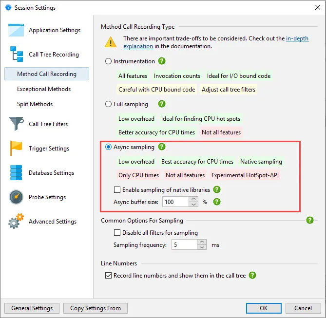
An async sampling mode without safe-point bias has been added on macOS and Linux. It uses the
non-standard AsyncGetCallTrace API in the HotSpot JVM to get call stacks at arbitrary times and not only
at certain execution states that the JVM considers as safe points. This profiling mode produces more accurate
CPU data for highly multi-threaded CPU-bound code.
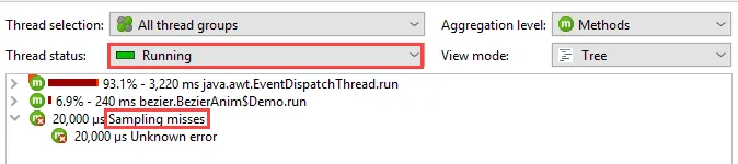
The only thread state that can be measured in this way is "Running". The waiting, blocking and net I/O thread
states are not available. Contrary to the other method call recording types that use a "Runnable" thread state
to measure when threads are eligible to be scheduled on the CPU, "Running" only measures times where a thread
is actually scheduled on the CPU. Obtaining the call stack can fail for a number of reasons which are
summarized in the "Sampling misses" top-level node.
Async sampling uses pre-allocated buffers that may be too small to capture all call stacks. This condition
is also shown in the call tree, and the session settings offer a way to increase the buffer size relative to the
default size.
Note that Windows does not have signal handlers and does not support this kind of data collection.
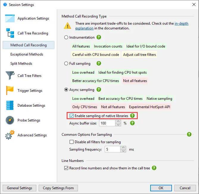
Native sampling has been added on macOS and Linux. When using the new async sampling mode described
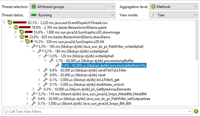
above, you can optionally enable native sampling. If native sampling is enabled, JProfiler resolves
symbols in native libraries and adds native nodes to the call tree.
In native call tree nodes, the associated native library is shown in square brackets followed by the
function name.
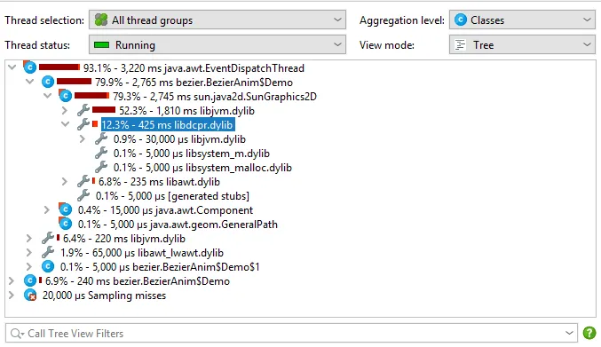
In the classes aggregation mode, native libraries are grouped together, while in the package
aggregation level all native calls are cumulated. When removing parts of the call tree, the library also
acts like a class, so by removing the class of the selected node (a new feature in this release that is
presented below), the entire native library is removed from the call tree.
JProfiler can now open JDK flight recorder (JFR) snapshots. JFR snapshots are often recorded in production
environments where the installation of profiling agents is restricted. Starting with this release, you can
now bring JProfiler's full arsenal of analytic features into play when analyzing these snapshots.
The available views in the view selector are different from those in a regular JProfiler sessions. JProfiler
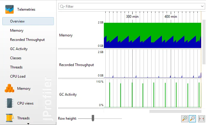
can construct a number of telemetry views from JFR event data including heap size, recorded throughput,
GC activity, class loading, thread counts and CPU load.
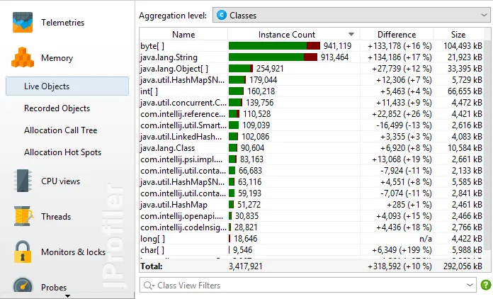
In the memory section, both heap statistics and allocation recording are shown. If heap statistics were enabled
for JFR recording, the "Live Objects" view shows the classes that took up most of the heap. The difference
between the first and the last heap statistics is shown in the "Difference" column.
Data from allocation recording
in JFR snapshots maps to the "Recorded objects", "Allocation Call Tree" and "Allocation Hot Spots" views.
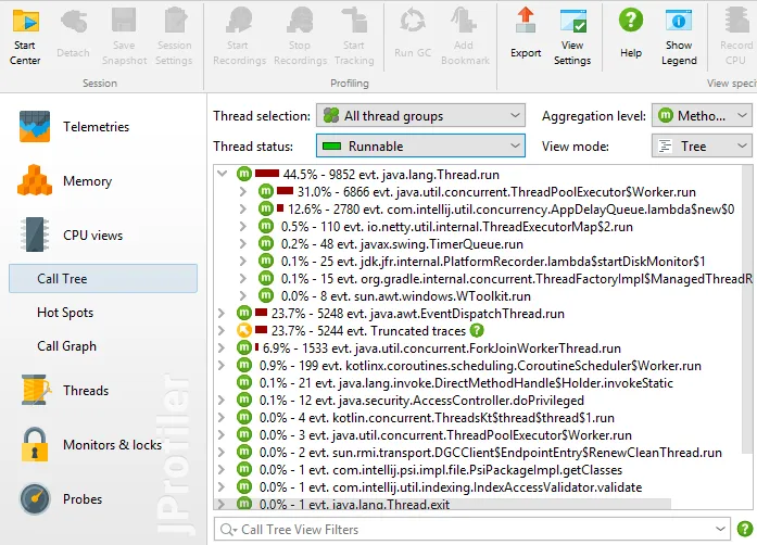
In the CPU section, "Call tree", "Hot Spots" and "Call Graph" views are available. JFR recording truncates
traces depending on buffer sizes, those traces are contained in a separate top-level node.
JFR recording only records threads that are runnable and in Java code. Due to the nature of JFR sampling, no
time calculation is possible and only event counts are displayed. The "Waiting", "Blocking" and
"Socket and file I/O" thread states show times because they are assembled from timed events.
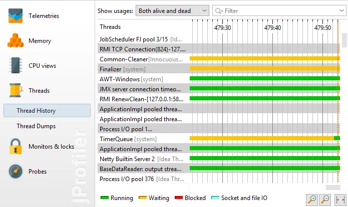
JFR snapshots contain thread data that JProfiler uses to build the thread history view. The contained thread
dumps are also displayed in JProfiler.
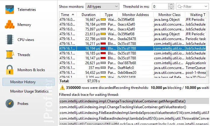
"Waiting", "Blocking" and "Parking" events from JFR snapshots are shown in the "Monitor History" view in the
"Monitors & Locks" section. These events are the sources of the "Waiting" and "Blocked" thread states in
the CPU views. The "Monitor Usage Statistics" view is also available.
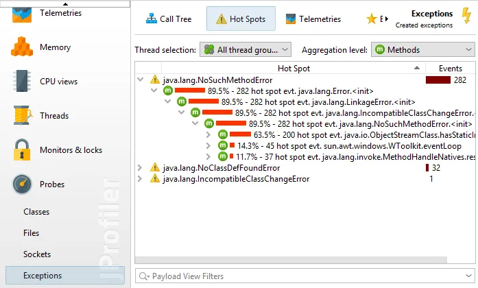
Finally, a number of probes are built from JFR events: "Classes", "Files", "Sockets" and "Exceptions". These
views show data depending on whether the corresponding JFR events were recorded. The "Files" and "Sockets"
probes are also the source of the "Socket and file IO" thread state in the CPU views.
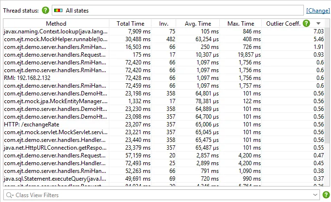
The new outlier detection view shows how the invocation times of methods vary with respect to their
average. Data for this view is always available when instrumentation is used for method call recording and
CPU recording is active. It replaces the "Method statistics" view which had a separate recording that
added a lot of overhead.
The outlier coefficient quantifies how much the maximum invocation times deviates from the average.
Methods with a high outlier coefficient are good candidates for inspection with the exceptional method run
recording feature in JProfiler that shows you their slowest invocations separately in the call tree.
Also, time measurements for outlier detection are performed for the same selected thread state as for
exceptional method run recording.
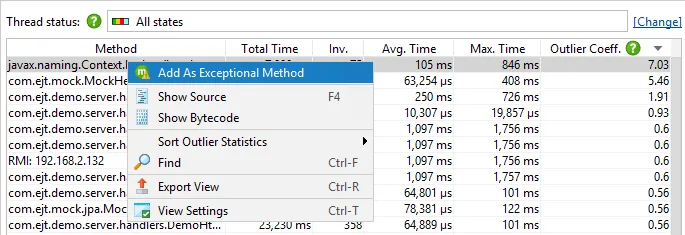
From the outlier detection view, you can easily select a method as an exceptional method in the context menu.
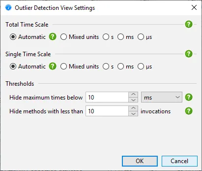
Thresholds for maximum times and invocation counts limit the amount of displayed data and can be adjusted
in the view settings.
Tracking of async calls now works with sampling, including the new async sampling mode. Previously,
you had to profile with instrumentation to use the "Inline async executions" call tree analysis. Having to
change the profiling mode to get inlined call stacks proved limiting, particularly for Kotlin coroutines,
where inlining is especially important.
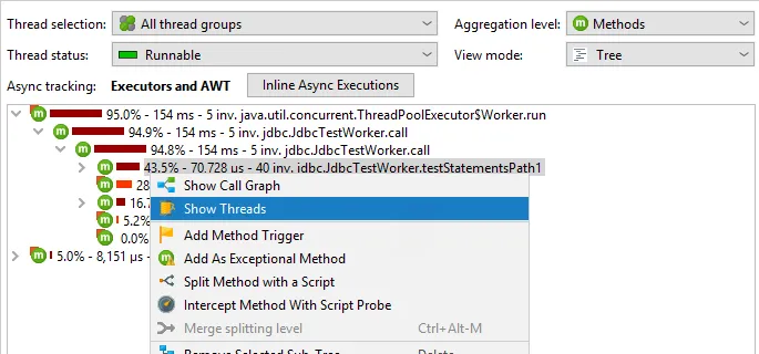
In the call tree you can now show all threads that contribute to the selected call stack. When
looking at the call tree cumulated for all threads, it can be interesting to know which single threads
are responsible for adding time to the selected node. The context menu gives you access to this action.
From the list of threads you can directly switch to a selected thread in the call tree.
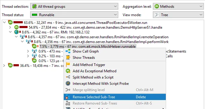
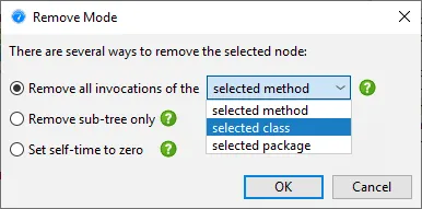
Call tree removal for entire classes or packages has been implemented. You can remove parts of the
call tree by selecting a node and choosing the "Remove selected subtree" action.
In addition to just removing the selected method, you can now choose to remove all invocations of the
selected class or the selected package.
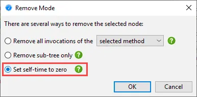
In some situations, you may want to keep the selected method, but just set its self-time to zero. For example,
this can be the case for the Thread.run top-level method where most of its self-time is in
non-profiled classes and you want the percentages of the profiled code to add up to 100%.
Telemetry drawing has been improved. When telemetries are zoomed out they now show the minimum
and maximum envelopes of jittery graphs instead of the interpolated average for each pixel. Also, peaks are
preserved for all zoom levels.
In addition, you can now zoom in and out with CTRL + scroll wheel or pinch gestures on macOS,
and telemetries will preserve the current cursor position when zoom levels are changed.
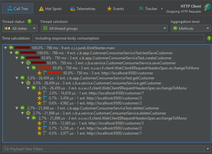
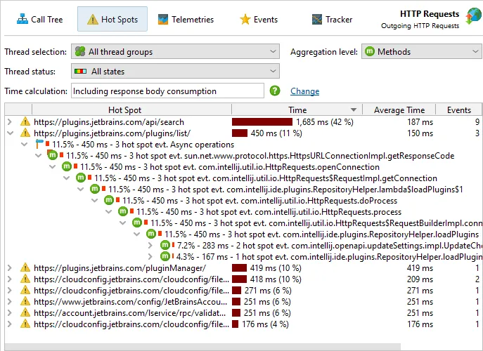
An HTTP probe for outgoing requests has been added. Both synchronous and asynchronous calls are
measured. The supported HTTP clients are:
- java.net.URLConnection
- Java HTTP Client (Java 11+)
- Apache HttpClient 4.x
- Apache Async HttpClient 4.x
- OkHttp 3.9+
- Jersey (JAX-RS) Async Client 2.x
- RestEasy Async Client 3.x
- CXF Async Client 3.1.1+
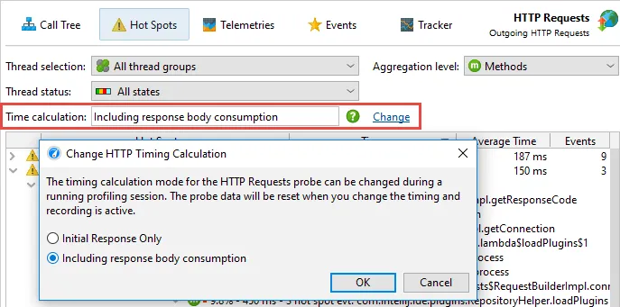
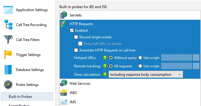
You can choose whether to include the consumption of the request body in the time measurement or stop
timing when the response code is available. This setting can be changed on the fly.
As with other probes, you can optionally annotate HTTP requests into the call tree view.
By default, the description of the HTTP request is the URL without the query, with an option
to retain the full URL for the probe events view. Optionally, you can configure a script that constructs
a description for the HTTP request which may be important to get useful hot spots.
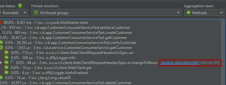
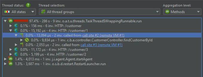
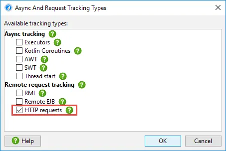
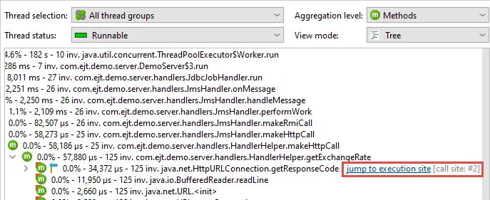
HTTP calls can now be tracked between JVMs. When using a supported HTTP client and a servlet
container on the server side, call sites and execution sites are navigable in both directions.
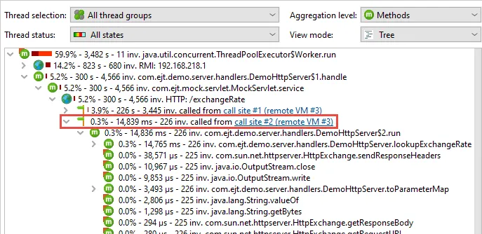
Call sites get a special icon and a hyperlink that shows the execution site in the server JVM
that must be profiled and open in a separate window for the navigation to work.
Execution sites are recorded separately for each call site so you can analyze different types of requests
in isolation. Each execution site is represented by a special node that is inserted into the call tree.
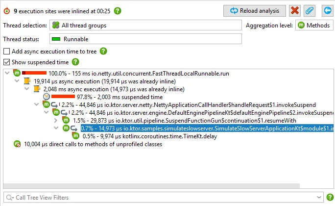
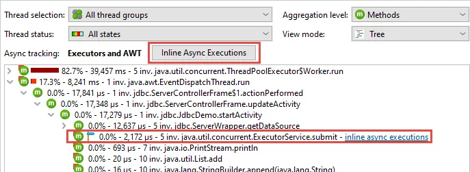
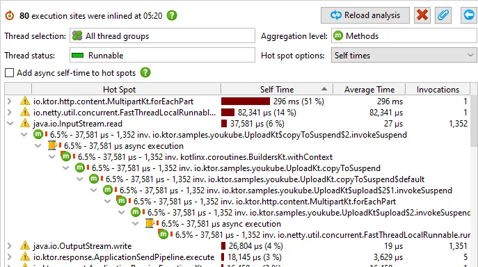
Async executions can be inlined. Both call tree and hot spots views now have an
"Inline Async executions" call tree analysis for this purpose. If async tracking is active,
a status display above the call tree provides easy access to the action that creates the inlined view.
Also, nodes in the call tree where an async call was intercepted have a corresponding hyperlink.
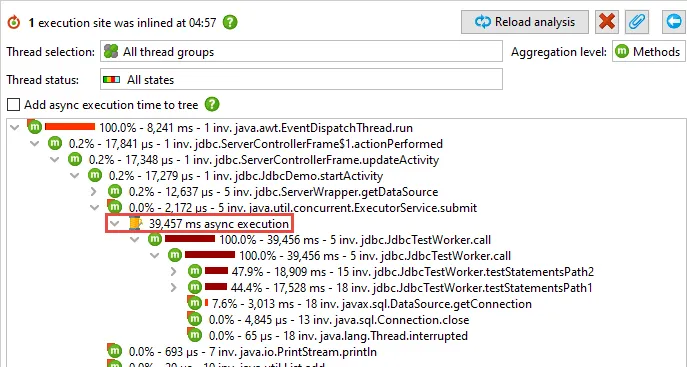
In the call tree analysis, "async execution" nodes show the call tree from the execution sites.
By default, the time below async nodes is not added to the parent nodes in the tree to show the non-blocking
nature of the calls.
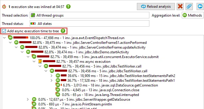
You can also choose to add the times as though the calls were blocking. This is useful for analyzing
which call stacks cause most time to be spent in the async execution sites.
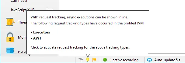
When async tracking is not activated, JProfiler detects which async tracking types have occurred in the JVM
and presents them to you in the status bar. With a single click you can then activate tracking.
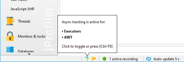
To quickly see which async tracking types are activated, hover the mouse over the status bar icon and click it
to invoke the configuration dialog.
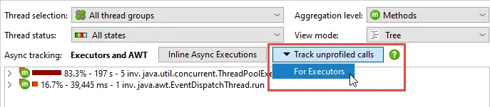
If async calls originate in unprofiled call stacks, they are not recorded by default in order to avoid
cluttering the analysis with framework internals. If such filtered async calls are detected, the async status bar
offers actions to switch on recording for these calls.
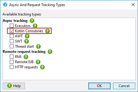
Support for tracking Kotlin Coroutines has been added.
Coroutines are the basis for
asynchronous programming with Kotlin in a multi-platform way. Without dedicated tool support, a call tree
involving coroutines is highly segmented and a lot of information about causality is lost.
When the tracking of Kotlin Coroutines is activated, the "Inline Async executions" call tree analysis produces
a call tree that shows call stacks across suspension boundaries. If applied to the hot spots view, the
call tree analysis shows you backtraces that would otherwise terminate at the first suspended method call.
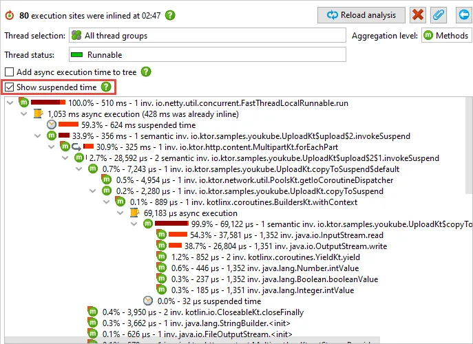
Kotlin Coroutine tracking also measures the times when coroutines are suspended and shows these times in separate
nodes in the inline call tree. This is needed to determine how long coroutine execution takes in total. If only
the actual processing times of coroutines are of interest, suspended times can be hidden.
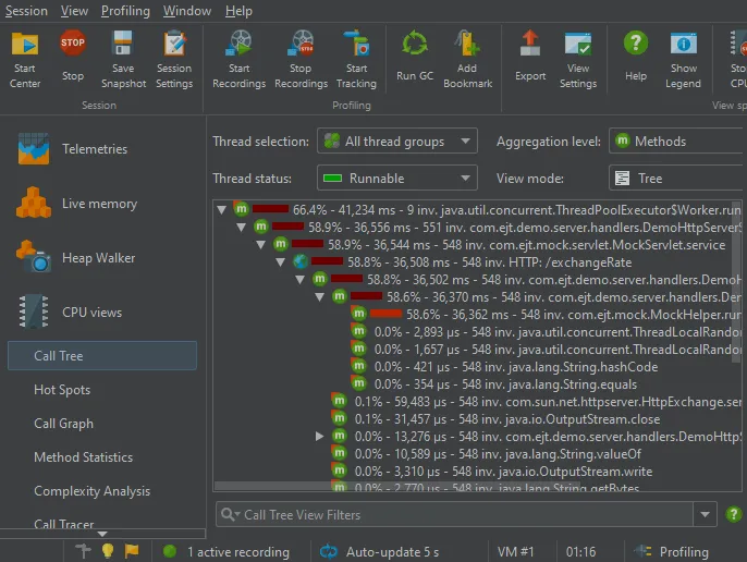
JProfiler has new light and dark look and feels. The look and feels are based on the
IntelliJ IDEA Darcula look and feel and its light
derivative. These look and feels support HiDPI on Windows, Linux and macOS. On Windows and macOS,
JProfiler is bundled with the "JetBrains Runtime" OpenJDK
that has better HiDPI support than the default JDK.
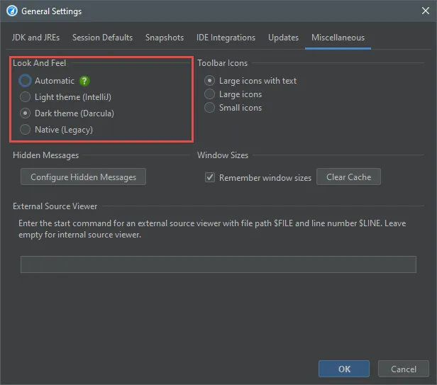
The default setting for the look and feel is now "Automatic", which chooses the dark theme if the OS is in dark
mode and the light theme otherwise. This detection is currently implemented on macOS 10.14+ and Windows 10 build 1809+.
A non-interactive mode for jpcontroller has been added. jpcontroller is a command line executable for
controlling recording and saving snapshots. In addition to the existing interactive mode, you can now also
automate profiling sessions without the need for manual input.
For an automated invocation, you pass [pid | host:port] to select a profiled JVM as well as the
--non-interactive argument. A list of commands is read, either from stdin, or from a command file that
is specified with the --command-file argument.
Commands for this non-interactive mode are the same as the method names in the
JProfiler MBean.
They require the same number of parameters, separated by spaces. In addition, a sleep <seconds>
command is provided.
For example, a command sequence could look like this:
addBookmark "Hello world"
startCPURecording true
sleep 10
stopCPURecording
saveSnapshot /path/to/snapshot.jps
Automatic detection of call tree filters for IDE integrations. For new sessions, the IDE integrations
for IntelliJ IDEA, eclipse, and NetBeans now scan the source packages of the profiled project and set inclusive
filters accordingly. Inclusive filters yield much better results than the default exclusive filters.
If all packages with editable source files have a common prefix package, that package will be used, otherwise
all top-level packages that contain classes will be added separately.
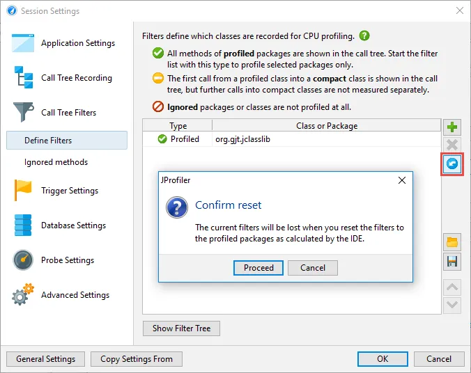
This detection will only be performed the first time a project is profiled, and any manual changes in the
call tree filter settings will not be lost. On the "Define filters" tab of the session settings dialog, you can
force this calculation to be repeated with the reset button.
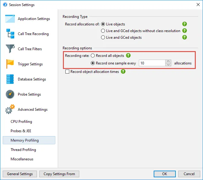
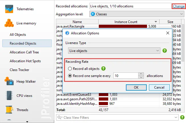
Sampling for allocation recording reduces the high overhead of allocation recording considerably.
By default, every 10th allocation is recorded which roughly reduces the overhead to 1/10th compared to
recording all allocations.
For live sessions, the sampling rate can be adjusted on the fly without losing any data.
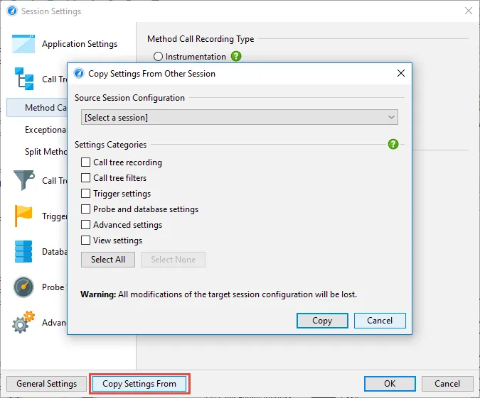
Session settings have been improved. The previously separate "Profiling settings" dialog has been integrated
into the new session settings dialog.
You can now easily copy selected parts of other sessions into the current session configuration.
There is now a default session that you can configure from the general settings dialog. All new sessions
start out with these defaults.
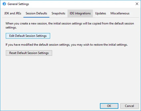
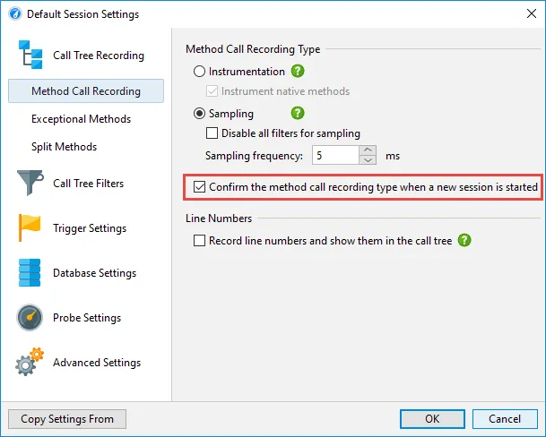
In the default session, you can now disable the initial question for new sessions whether
sampling or instrumentation should be used.
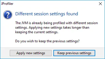
If you connect to a JVM is already profiled with different session settings, JProfiler will give you the option
to keep the previous session settings. These previous settings can be inspected in the session settings
dialog after the profiling session has been started. This mechanism eliminates time-consuming class
retransformations.
Applying profiling settings at startup without using the JProfiler UI has been made more convenient.
When using the "id" or "config" options in the -agentpath VM parameter, you no longer have to specify the
"nowait" option which is now implied. The "id" option is no longer necessary if the config file only contains
a single session. A typical VM parameter for profiling will now look like this:
-agentpath:/opt/jprofiler/bin/linux-x64/libjprofilerti.so=config=~/jprofiler_config.xml
The ~ character is now replaced with the home directory on all platforms, and the default name of the JProfiler
config file has been changed to jprofiler_config.xml in order to make it less generic.
When configuring profiling sessions on remote machines or offline profiling sessions without the JProfiler UI,
it is sometimes necessary to inspect the config file and make manual changes. In this release,
the config file format has been improved making it less verbose by omitting default settings and
making all aspects of the configuration easily understandable.
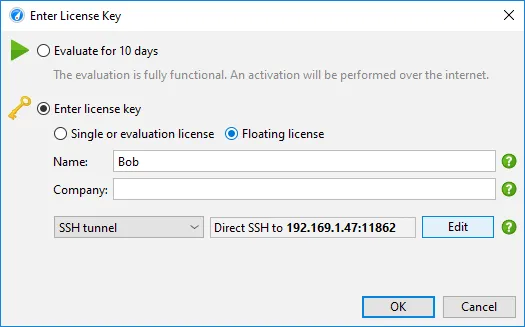
Floating licenses now work over SSH. Customers with floating licenses can now configure an SSH connection
to the floating license server using the same configuration as for SSH connections to profiled JVMs.
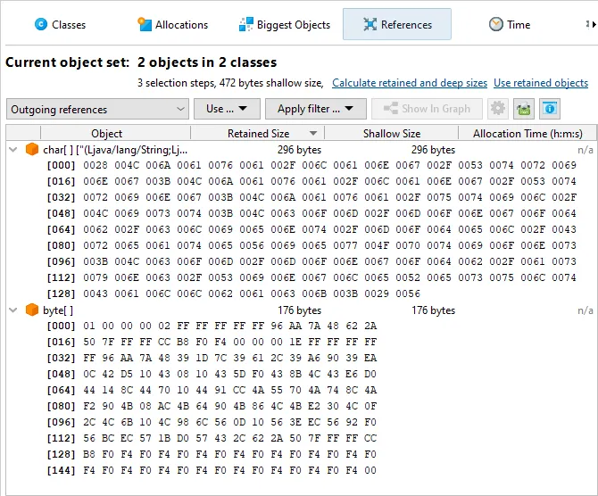
A tabular display of char and byte arrays has been added in the outgoing reference view of the heap
walker. Larger amounts of data can now be interpreted much more easily.
In addition, char arrays now show their string value right next to the instance.
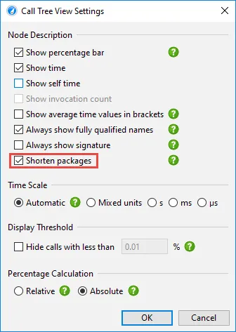
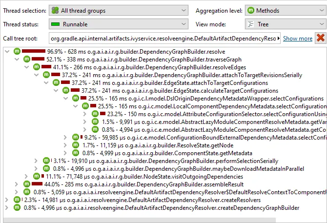
Shortened package names in call trees have been implemented. This optional setting is configurable
in the view settings dialog.
For code bases with deep package structures, the shortened package names reduce the amount of displayed text
and make it easier to focus on class and method names.
Improved support for IBM and OpenJ9 JVMs. This release brings feature parity with HotSpot JVMs in
a number of areas:
- Support for primitive data in the heap walker
- All inspections in the heap walker are now supported
- File and process probes are supported for IBM 8+ JVMs
- The "Save HPROF snapshot" UI action and "Create an HPROF heap dump" trigger action now generate PHD dumps
Support for profiling Java 12+. Also, all OpenJDK variants are now supported when starting sessions
from the JProfiler UI.