JProfiler 14.0 introduces the following notable new features:
JProfiler 14 adds full support for profiling Java 21, including virtual threads.
Java virtual threads are thread-like tasks that aim to revolutionize high-scale concurrency on the JVM.
All aspects of JProfiler have been reworked so that profiling millions of virtual threads causes minimal overhead.
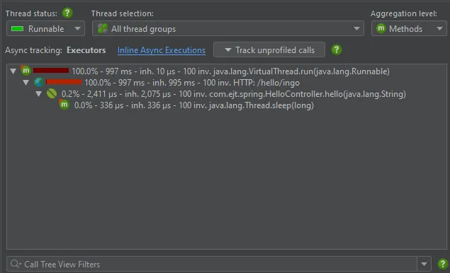
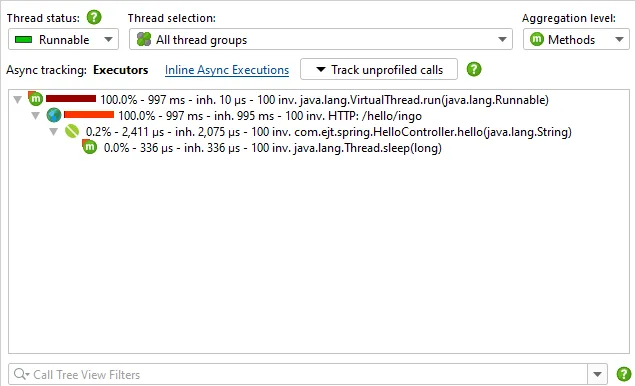
In the call tree, virtual thread executions will have a top-level node of java.lang.VirtualThread.
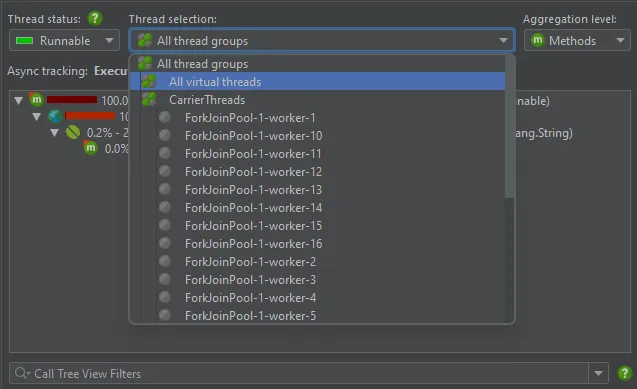
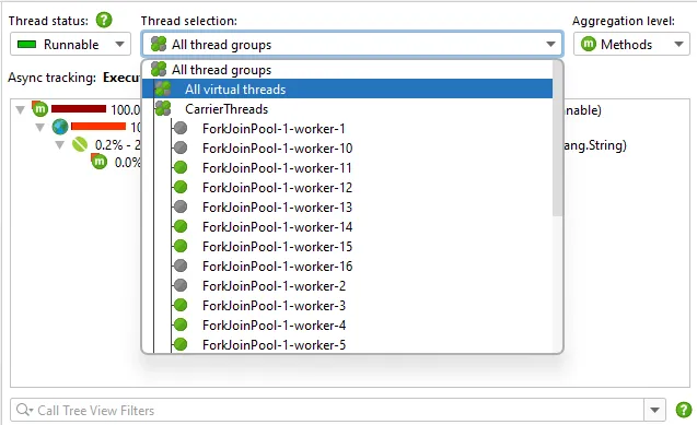
Virtual threads are not recorded separately like platform threads, so all virtual threads are contained together in a single synthetic
thread group.
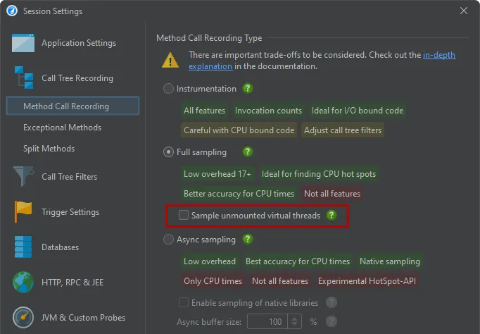
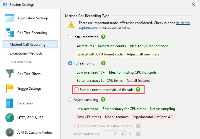
By default, only mounted virtual threads are sampled. This means that blocking states of virtual threads are not captured by CPU recording.
For debugging purposes, there is an option in the profiling settings to sample unmounted virtual threads.
Like for platform threads, JProfiler supports async tracking for the creation of new virtual threads. If enabled, the
"Inline Async Executions" call tree analysis connects call sites with execution sites. In this case, the call site is the last profiled
method before the VirtualThread instance is created. The execution site is a top-level node in the started virtual thread.
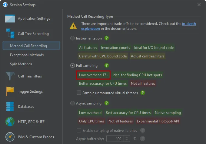
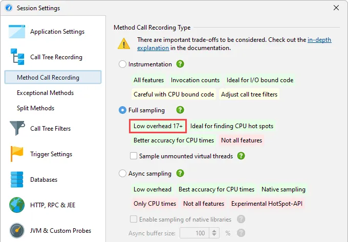
Near-zero overhead for full sampling when profiling Java 17+. Using new facilities in the JVM, JProfiler can now perform sampling
with a negligible overhead, even for heavily multi-threaded applications where the overhead for sampling used to be significant.
From an overhead perspective, sampling is now on equal terms with async sampling if you profile Java 17 or higher.
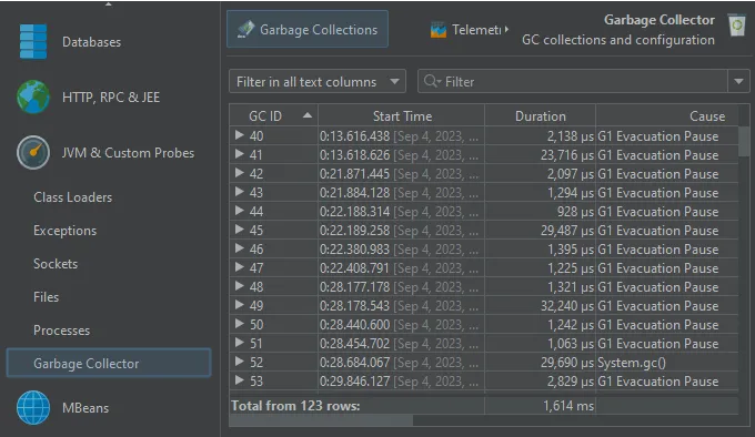
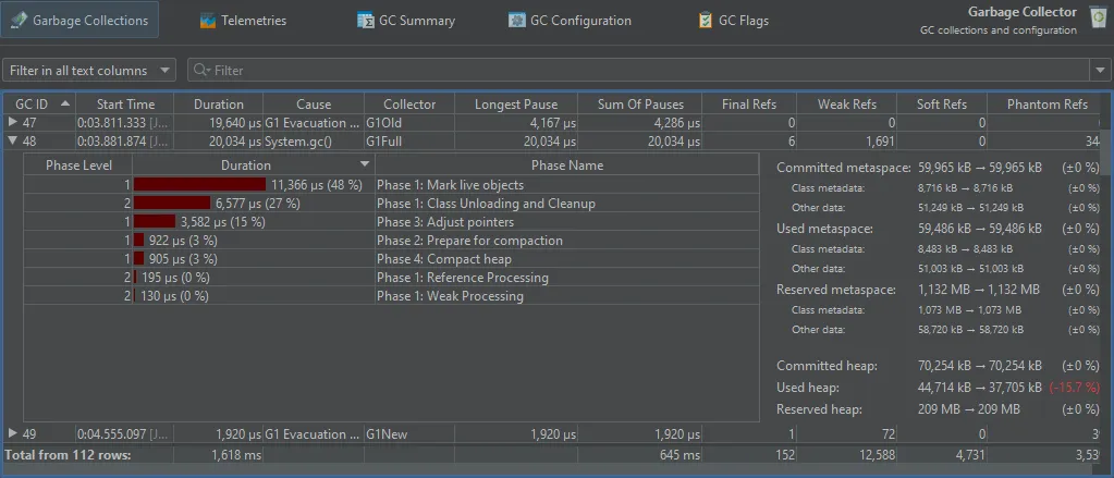
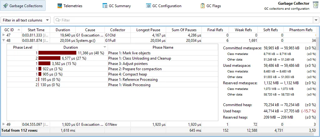
A garbage collector probe was added. The GC probe is available when profiling Java 17+ and shows detailed data about single garbage
collections and the GC configuration.
Because of the increasing number of probes, the probe sections have been reorganized and the GC probe can be found in the new
"JVM & Custom Probes" section.
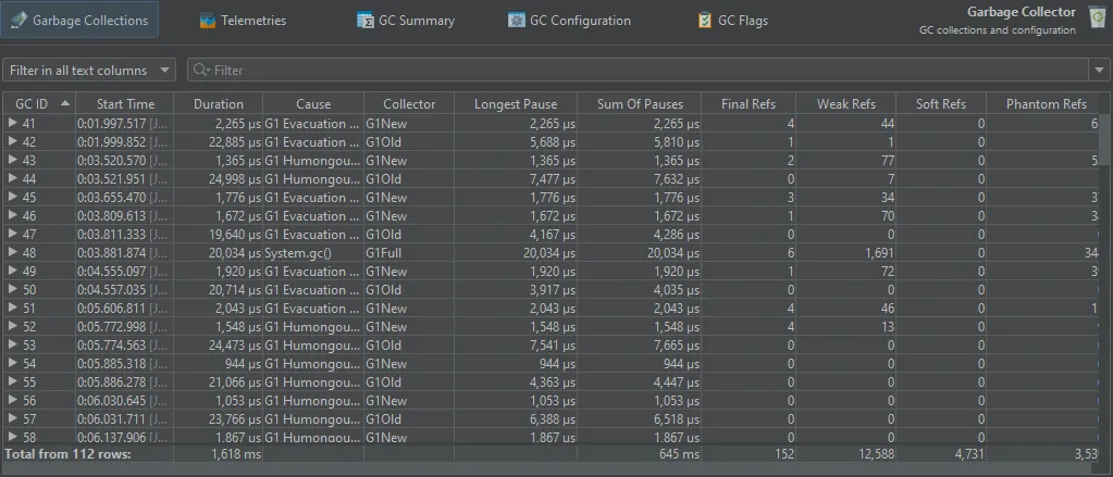
Its main view is the "Garbage collections" view that shows single garbage collections in tabular form. It shows you the triggering cause,
how long the collection took, how many references were collected and what pauses were caused by the garbage collection.
If you need even more detail, each garbage collection can be expanded to show the single phases with their duration. To the right of the
GC phase table, statistics about the changes in heap and metaspace are shown.
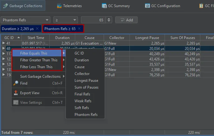
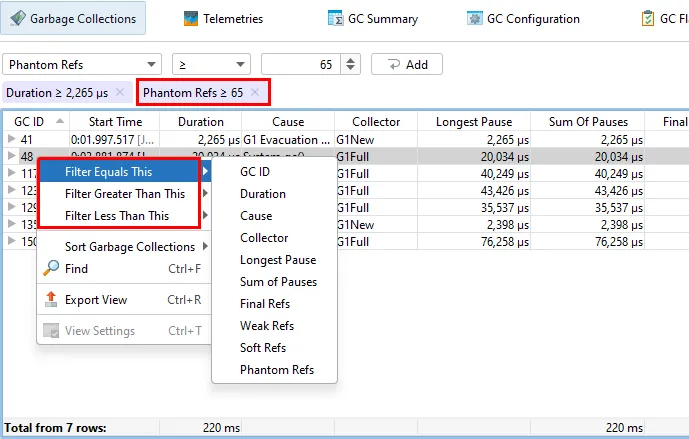
To help you analyze important garbage collections, you can set multiple filters, most conveniently with the context actions on the
garbage collections table and the phase table. Filters are added as tag labels above the table and can be removed by clicking their close button.
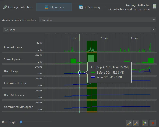
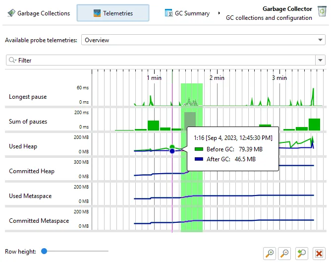
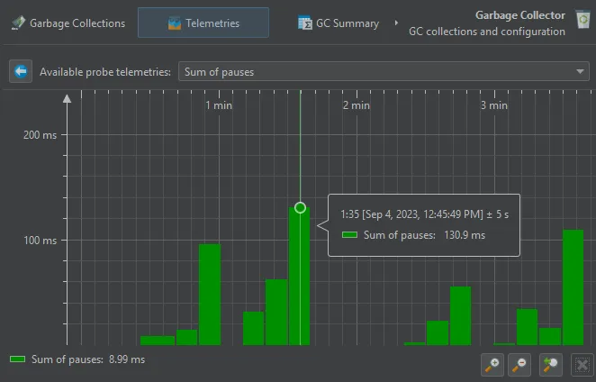
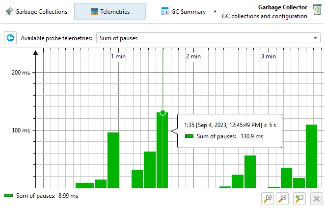
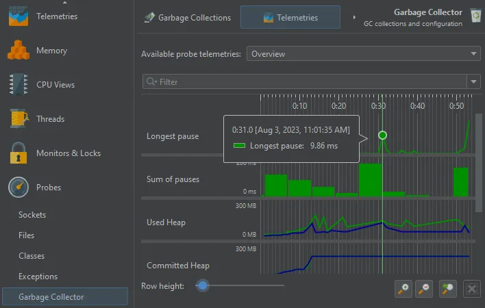
The GC probe produces a number of GC telemetries which are available in the "Telemetries" probe view.
If you are interested in minimizing GC pauses, the "Longest pause" telemetry at the top will be the most interesting one.
You can drag along the time axis of the telemetry to select the corresponding garbage collections in the "Garbage Collections" view.
For better vertical resolution, you can select a single telemetry from the drop-down at the top or by clicking on the name of the telemetry.
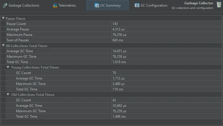
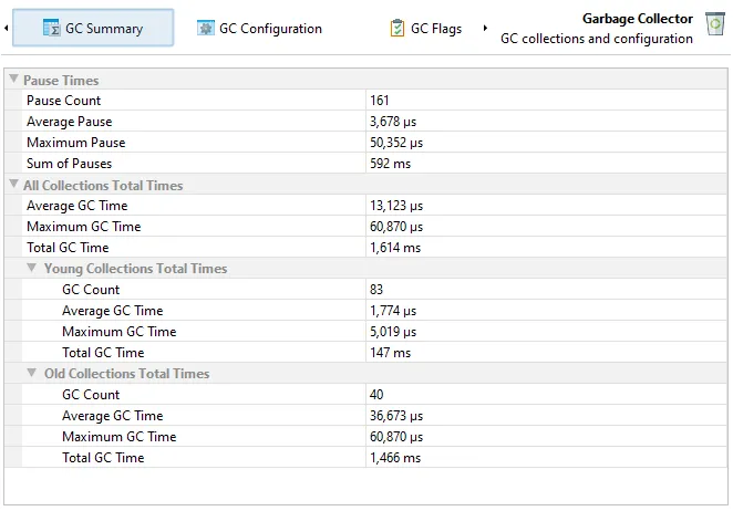
The GC summary view shows you measurements that are aggregated over the entire recording period. Each measurement provides the number
of garbage collections, as well as the average, maximum and the total values. The most important data at the top are the "Pause times"
that directly affect the liveness of your application.
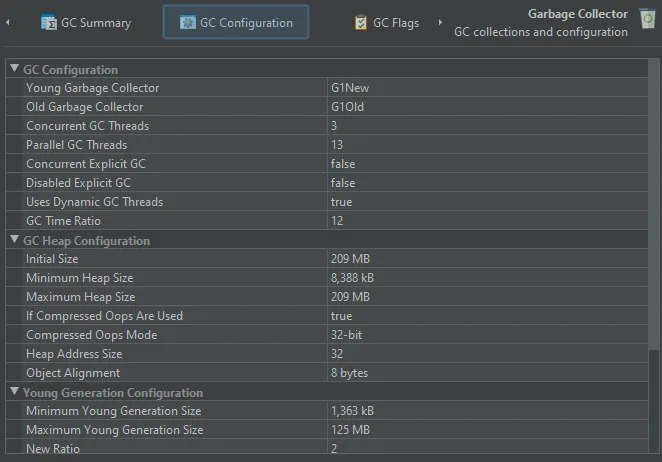
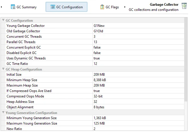
In the GC configuration view, you can inspect the common properties that can either be set explicitly or that are set
implicitly by the garbage collector itself. These properties are common to all garbage collectors and help you understand the
differences between garbage collectors.
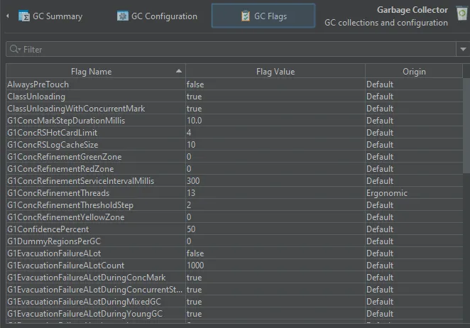
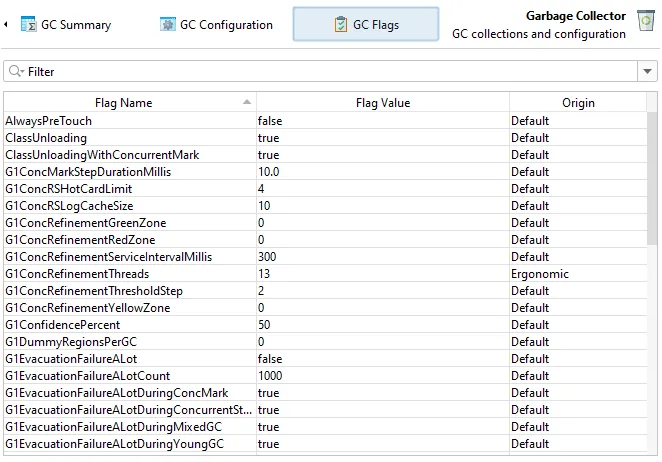
Finally, the GC flags view gives you an idea what properties of a garbage collector can be tuned and lets you check their actual
values. The "Origin" column shows you how the flag was set.
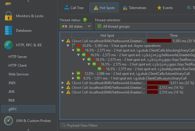
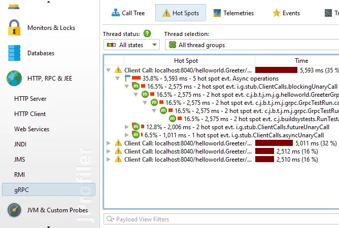
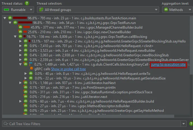
A gRPC probe has been added. gRPC is a popular RPC framework that uses HTTP/2 and Protocol Buffers, offering features like
streaming and multiplexing. This probe can be found in the new "HTTP, RPC & JEE" probe section.
JProfiler can track remote gRPC calls between JVMs if gRPC remote request tracking is enabled.
You can then see hyperlink labels in the call tree view for incoming and outgoing calls that will take you to the corresponding
call tree location. This requires that both JVMs are profiled in separate windows or snapshots are opened that were recorded during the
remote call.
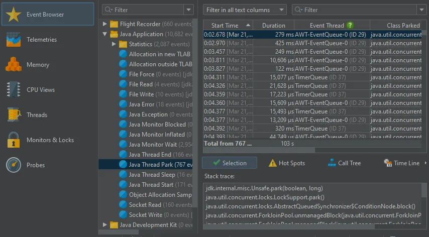
JProfiler 14 adds first-class support for JDK Flight Recorder (JFR) snapshots. The centerpiece of this support is the
new JFR event browser.
JFR is a structured logging tool that records a broad range of system-level events. Similar to the black box of an aircraft that
continuously records flight data for use in incident investigations, JFR continuously records a stream of events in the JVM for use
in diagnosing problems.
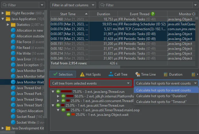
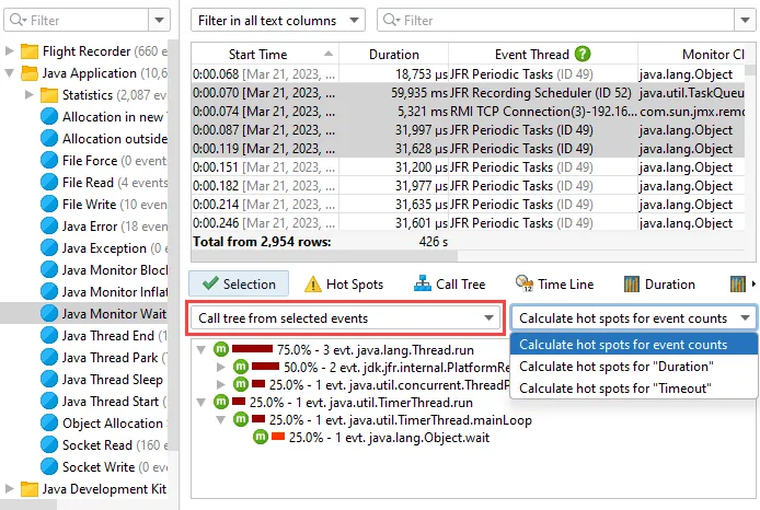
Events are categorized hierarchically and shown in the tree on the left side, single events are displayed in the
table on the right. The columns of the event table and the analysis views below it depend on which event types have been selected.
In the selection area, the stack trace of the selected event is shown if it was recorded. If you select multiple events, a call tree or
a hot spots view is shown for them. If the selected event types have time, memory or frequency measurements, you can choose to calculate
the hot spots for any of those measurements.
To avoid overloading the UI, the event table only shows a maximum of 10000 events. The analysis views operate on all events in the snapshot.
Due to the nature of JFR recording, JFR snapshots can become very large, so JProfiler's event browser has been optimized for maximum speed
even for extreme file sizes.
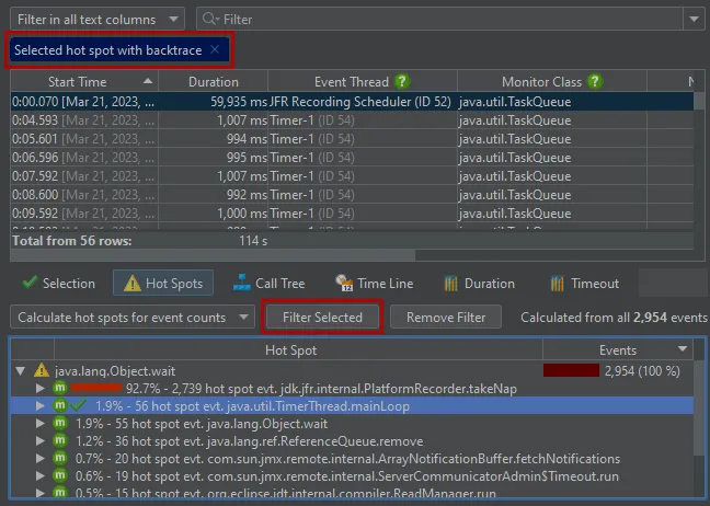
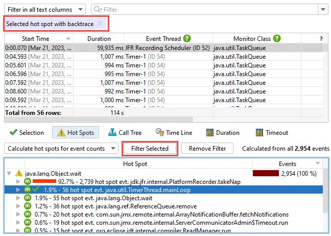
The "Hot Spots" and the "Call Tree" views are like their counterparts in the "Selection" area, but for all events of the selected event
types. Also, you can add call stack filters and hot spot filters and an optional back trace part.
Any analysis view itself is calculated from all filtered events, but excluding the filter that was set in the analysis view itself.
This makes the analysis view more useful because you can see what part of the total event set you have selected there.
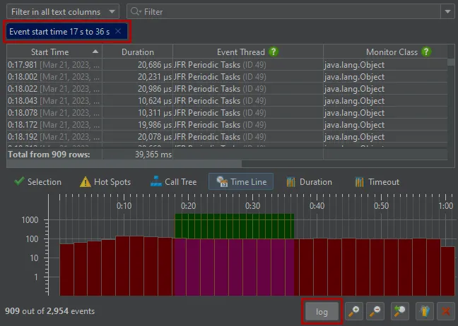
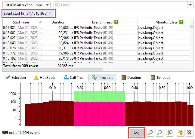
The "Time Line" view shows a histogram of all event start times. You can select a time range with the mouse and filter the events
in the table. By default, the view has a logarithmic vertical axis.
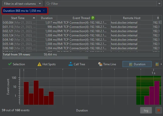
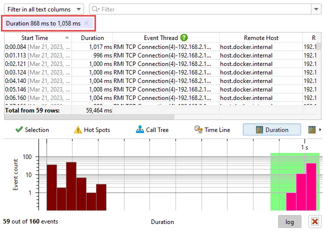
For each event column that contains a durations, memory sizes or a frequency, JProfiler adds a histogram view.
Histograms show event counts on their vertical axis while the horizontal axis shows the selected measurement. Bin sizes and event counts
are available from the tooltip. Event filters can be added in histogram views by selecting a range on the horizontal axis.
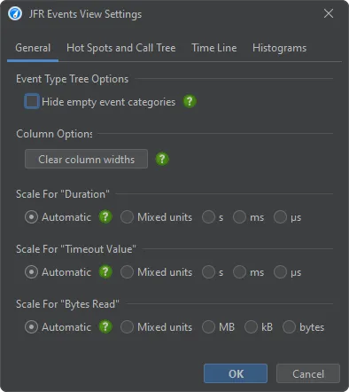
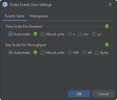
The view settings dialog of the event browser allows you to customize the views. For example, the scales for the columns that are currently
shown can be adjusted there.
Apart from the JFR browser, a subset of JProfiler's views that match with data provided by JFR are available when opening snapshots.
This is a capability that JProfiler already had before. In addition, the new garbage collector probe is now available for JFR snapshots.
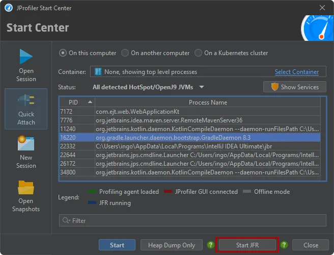
Along with the first-class support for opening JFR snapshots, JProfiler adds support for recording JFR snapshots directly
from within JProfiler.
In the attach dialogs where you can attach to a JVM for profiling, you alternatively start JFR recording. This includes all remote
connection capabilities of JProfiler, such as Windows services, SSH connections, Docker containers and Kubernetes.
Even if you are not interested in any particular JFR data, this recording mode can be useful if you are trying to obtain information
about a production environment where a native profiling agent that uses the JVMTI may not be loaded. JFR snapshots can contain
data about the runtime characteristics and even allow you to detect a pronounced CPU hot spot.
This is similar to the adjacent "Heap dump only" option that takes an HPROF memory snapshot without loading the profiling agent.
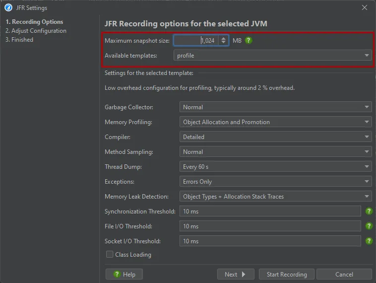
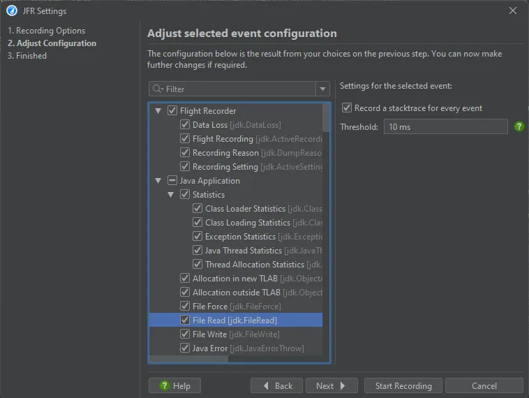
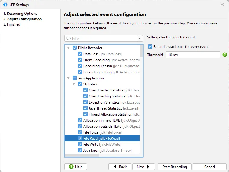
When you start JFR recording, a wizard is shown that lets you choose the JFR recording settings.
To avoid that the JFR recording fills up your entire hard disk, a maximum snapshot size has to be set. If exceeded, old chunks of data are
discarded.
JFR configurations files are located in the "lib/jfr" directory of the JRE. They contain a high-level configuration scheme that is shown as
a UI by JProfiler on the same wizard step.
In the next step of the wizard, the result of this configuration is shown as a tree of all JFR events. If you have already profiled this
JRE before, JProfiler will offer you to use the last settings.
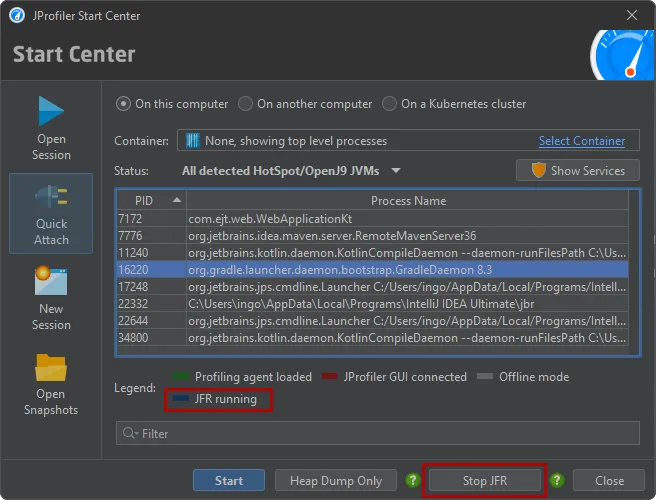
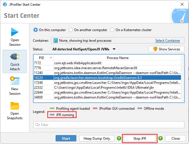
After recording is started, the JFR recording button changes to show "Stop JFR". Also, the background color of the unselected JVM entry in
the table changes to show that a JProfiler JFR recording is running.
After clicking "Stop JFR", the JFR snapshot is transmitted to the local machine and opened in JProfiler. These snapshots are temporary. If
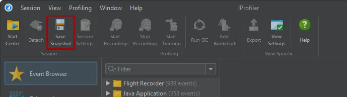
you want to keep the snapshot for later analysis, you can save them with the "Save snapshot" action.
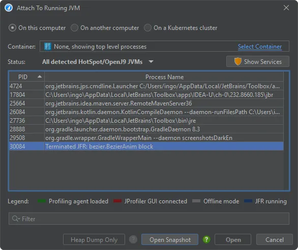
If a JVM where you have started a JFR recording in JProfiler terminates before you open it, the attach dialog will have a "Terminated JFR"
entry for it, and you can use it to download the JFR snapshot that the JVM saved at exit.
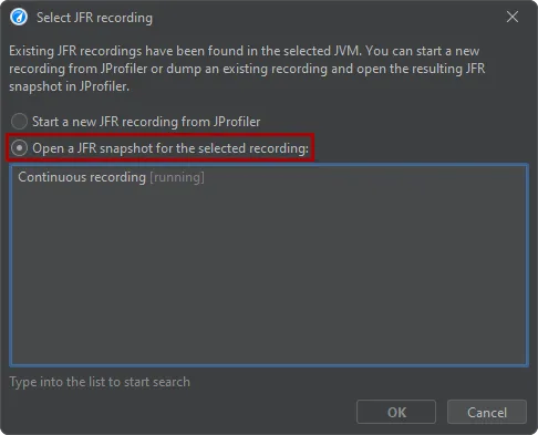
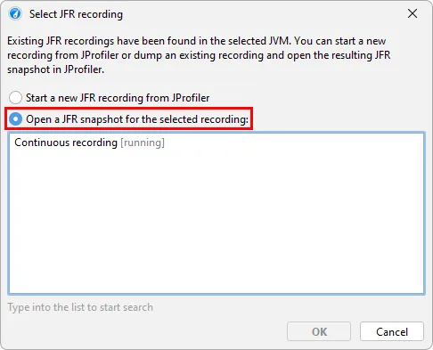
If JFR recordings are running in a JVM that were not started by JProfiler, you can still open them in JProfiler. In that case, JProfiler
will not show the recording wizard when you click the "Start JFR" button but a dialog where you can choose whether to start a new recording
or open an existing JFR recording. Existing recordings will never be stopped by JProfiler.
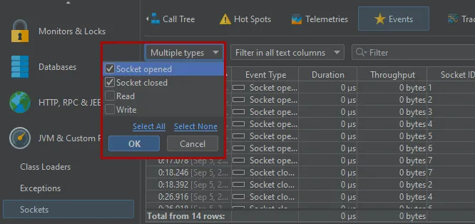
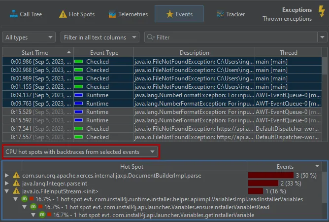
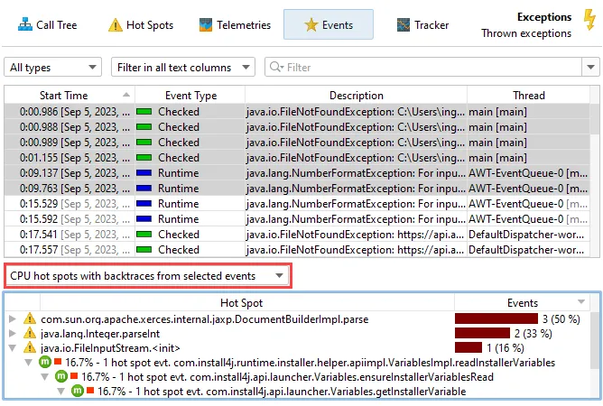
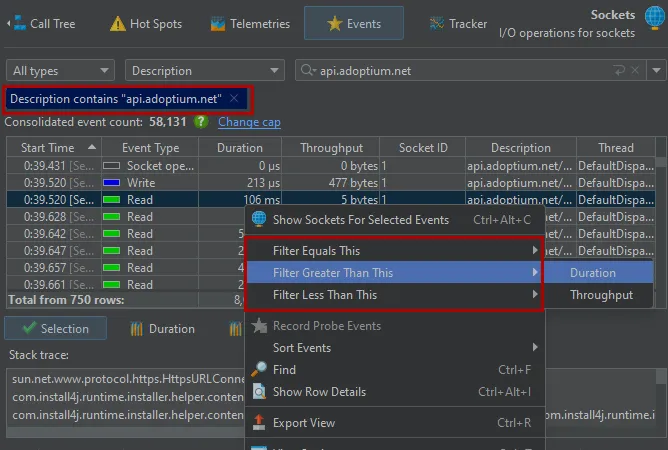
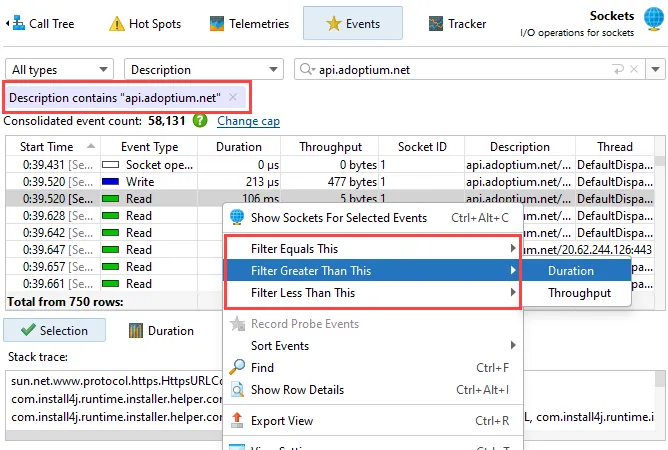
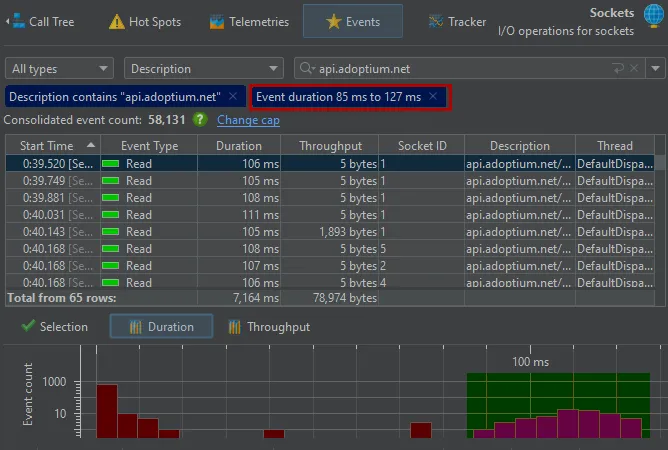
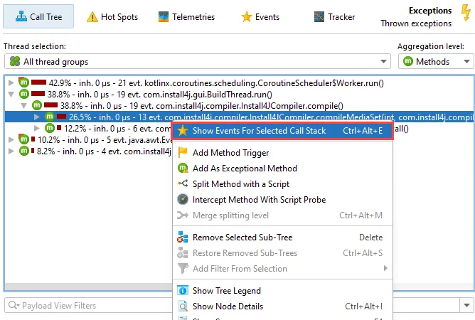
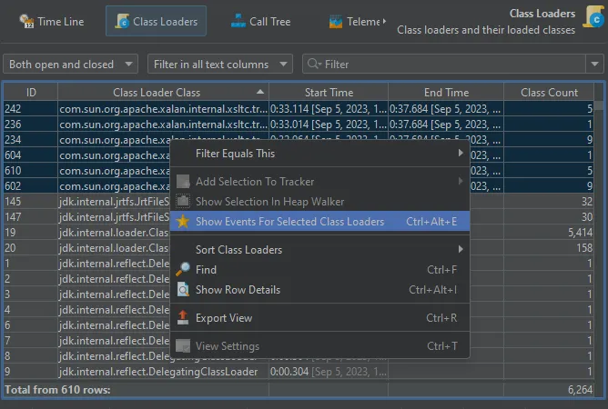
The probe events view has been improved in many ways. This view is part of nearly all probes.
Many probes handle a number of different event types at the same time. The type selector above the events table now allows you to
select multiple event types. For example, in the "Sockets" probe, you can now analyze when sockets were opened and closed without
getting distracted by the intervening "Read" and "Write" events.
When you select multiple events, the stack trace view at the bottom now shows cumulated data. For example, you can see
the CPU hot spots of the selected events with backtraces.
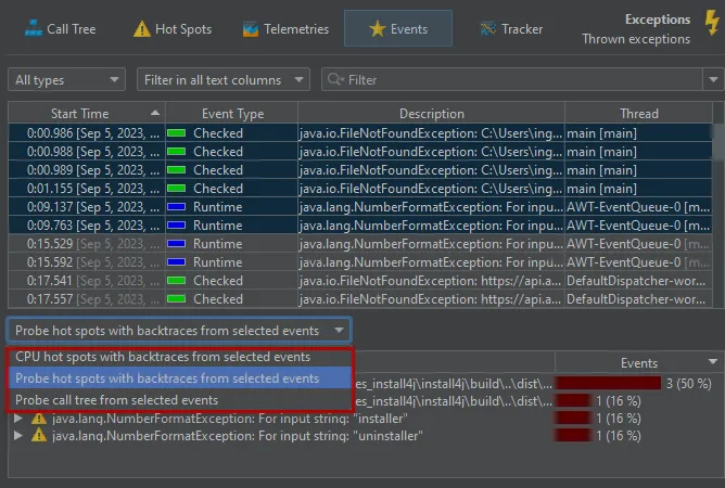
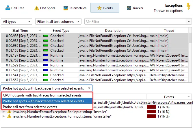
The other available views are the "probe hot spots with backtraces" that have the payload at the top and the "probe call tree".
Scales for durations and throughputs can now be adjusted in the view settings dialog of the probe events view and the control objects
view. These settings are saved separately for each probe.
Filtering in the probe events and the control objects views now works on a per-column basis. You can add multiple filters at the same
time, either at the top of the table or most conveniently from the context menu, in order to use a value in the selected row. Filters are
added as tag labels above the table and can be removed individually by closing them.
The probe events view now includes a histogram view for event durations and optionally a histogram view for throughputs if
the probe measures memory. By default, the views are logarithmic, so you can easily spot outliers. By selecting a value range on the
horizontal axis, you can add a filter for the probe events table.
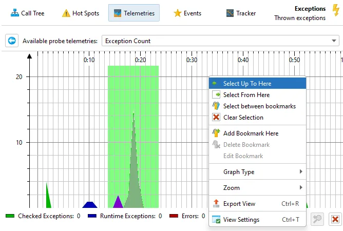
You can now filter probe events by selecting a time range in the probe telemetry views. You can do that either by dragging the mouse
or by using one of the selection actions in the context menu.
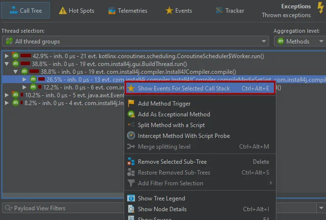
Probe event filters can now be set from the probe call tree and the probe hot spots view. The context menu in both tree views
as well as the tool bar has an action to create a filter and switch to the probe events view.
Multiple control objects can now be selected and the associated events can be shown. This allows you to analyze events for an entire
category of control objects.
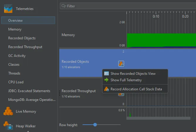
VM telemetries have been improved.
You can now drag and drop VM telemetries in the overview to change their order. This is useful to compare telemetries of interest. The
change in the order is persistent across profiling sessions and is reflected in the view selector on the left.
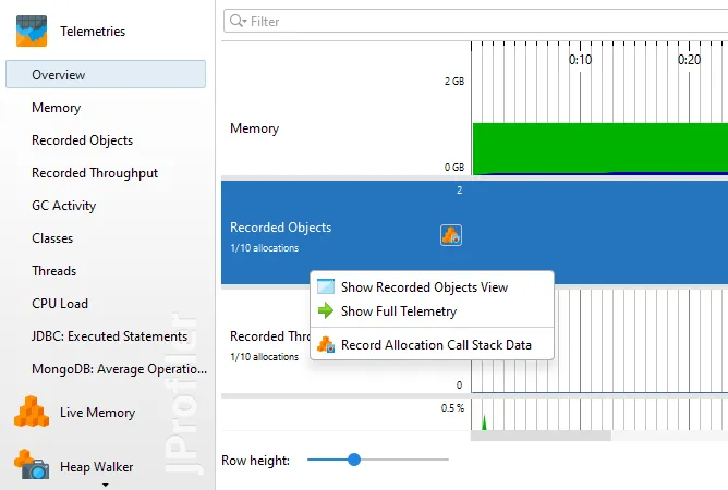
Also, the telemetries from the recorded object views are now always visible, even if no allocations are recorded. In that case, you
will see an inline recording button that lets you conveniently start allocation recording. The context menu also includes the recording action
if you want to stop it again that way as well as other actions to show the recorded objects view or the full telemetry.
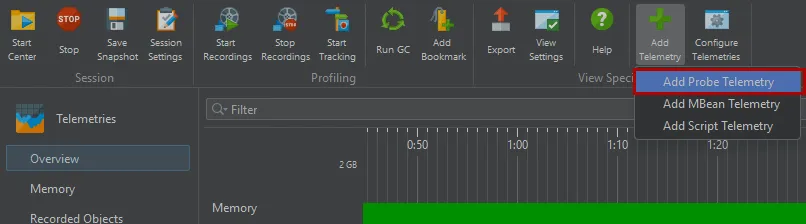
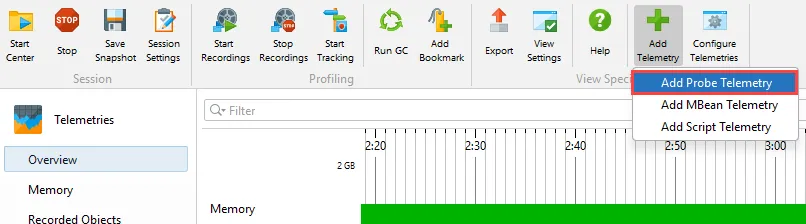
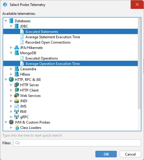
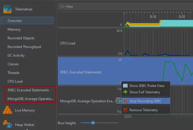
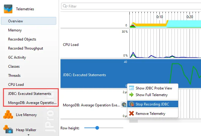
Probe telemetries can be added to the VM telemetries section. Previously, you had to activate a probe and navigate to its telemetry
view to see one of its telemetries. This made it difficult to compare them with the system telemetries or with telemetries from other probes.
Now you can configure a session to include any number of probe telemetries directly in the VM telemetries section.
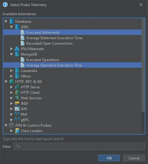
In the probe telemetry registry dialog, all available probe telemetries are listed and you can select multiple telemetries at once.
The probe telemetries are added at the bottom, but can be dragged to the desired index in the VM telemetries overview.
Like the telemetries from the recording actions, probe telemetries have an inline recording button if recording is currently stopped, and
the context menu allows you to navigate to the probe view.
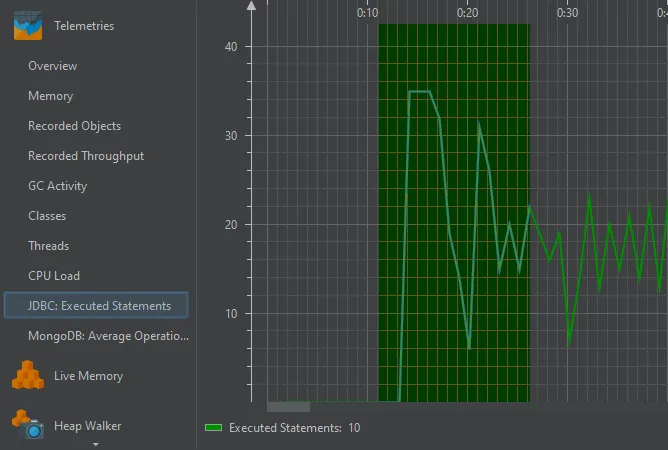
In the full probe telemetries, you can select a time range to create a filter in the probe events view, just like in the probe view itself.
After such a selection, the probe events view will be shown.
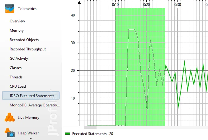
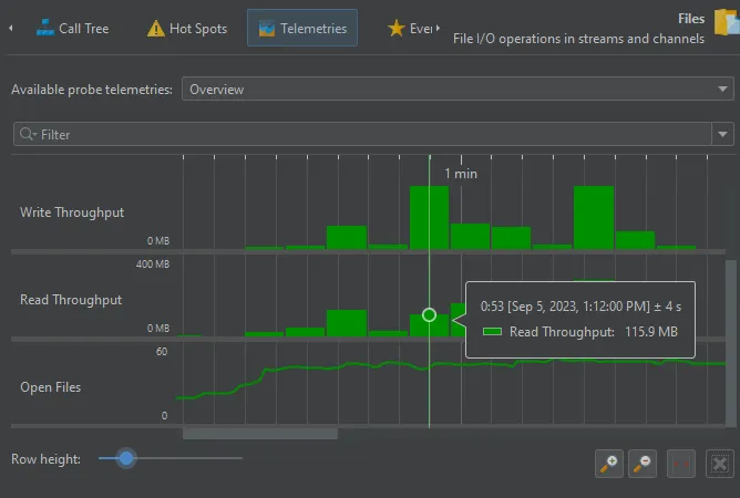
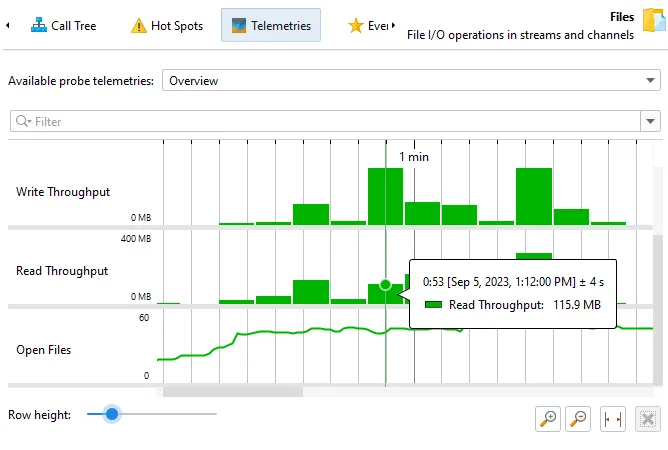
Telemetries that show rates are now shown as histograms. For example, this includes the recorded throughputs in the "Files" probe.
Previously, these telemetries were shown as line graphs which did not give a sense of the total throughputs when looking at time periods
much larger than a minute.
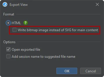
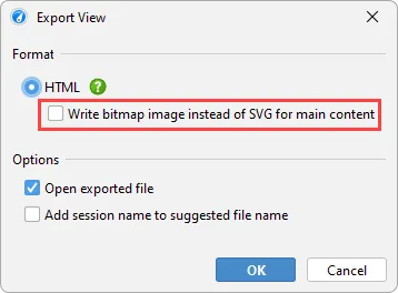
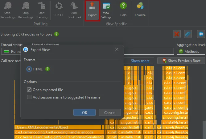
Finally, any telemetry can now be exported as SVG. The bitmap export is optionally still supported.
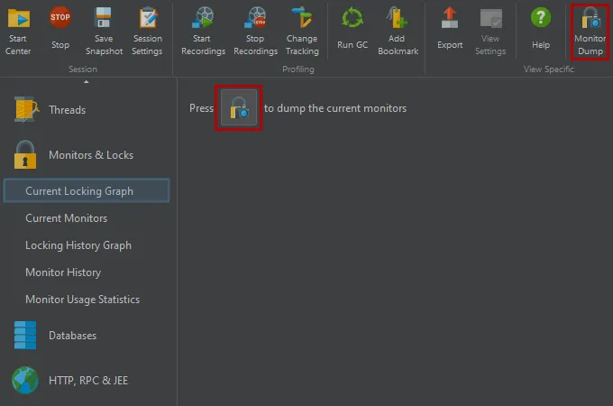
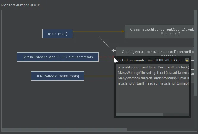
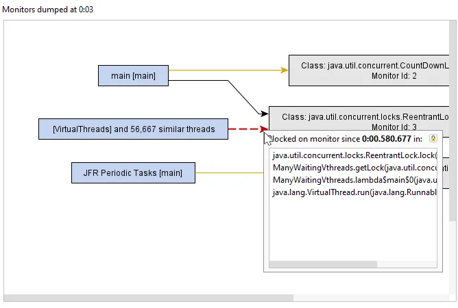
The current locking graph and current monitors views have been improved. These views are principally used for analyzing deadlocks.
Current monitor data is now a snapshot rather than continuously updated. This makes it easier to analyze a single locking situation.
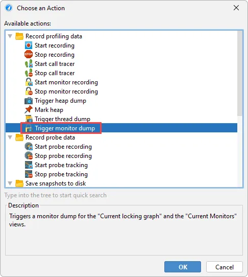
There is an action in the toolbar to dump the current monitors.
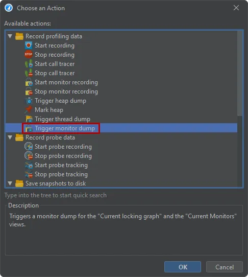
The current monitor snapshot also makes it possible to save this information in a JProfiler snapshot or to time the monitor snapshot
programmatically. There is a new method in the controller API as well as a trigger action for this purpose.
Current monitors and current locking graph views now show java.util.concurrent locks. In attach mode, these views are now
available, but only for java.util.concurrent locks.
Current monitors and locking graph views now group similar threads. This makes it easier to interpret locking situations with many
threads and is important for supporting virtual threads where large numbers of threads may be active at the same time.
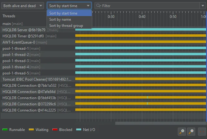
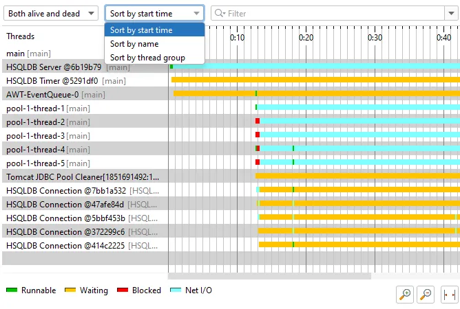
The thread history view and the probe timeline views now support reordering. You can drag threads or control objects to their desired
location or use the sorting drop-down to order the view by start time, by name or by thread group.
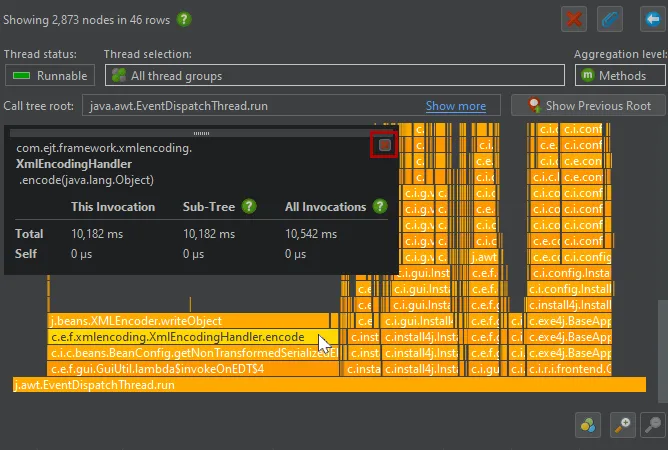
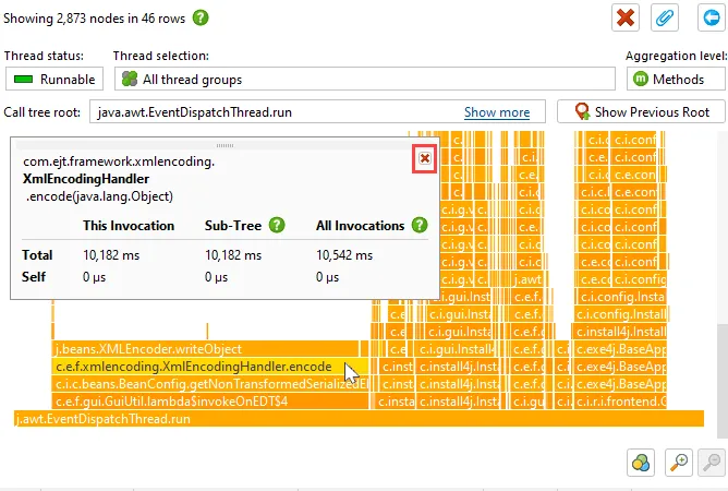
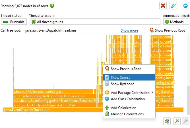
Flame graphs have been improved. Flame graphs are available in call tree views from the "Analyze->Show Call Tree" action.
When inspecting the nodes in the flame graph by hovering over them with the mouse, the tooltip can get in the way and obscure part of the flame
graph that you might want to look at. Now you can use the pin button in the top-right corner of the tooltip to move the tooltip to a
fixed location with the gripper at the top. The pin button then becomes a close button.
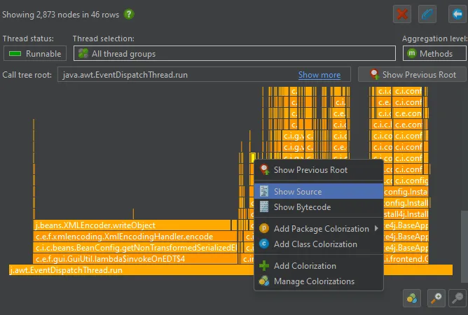
A "Show Source and a "Show Bytecode" action have been added to the context menu in the flame graph. As all such actions in JProfiler,
the "Show Source" action will open the source file in the IDE if you are using an IDE integration.
Flame graph colorizations are now persisted, so you don't have to configure them each time again for new profiling sessions.
Finally, flame graphs can now be exported as SVG. The exported SVG has basic tooltips so you can see the method names and their times.
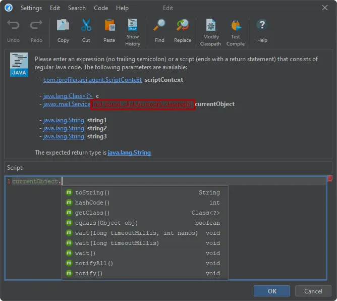
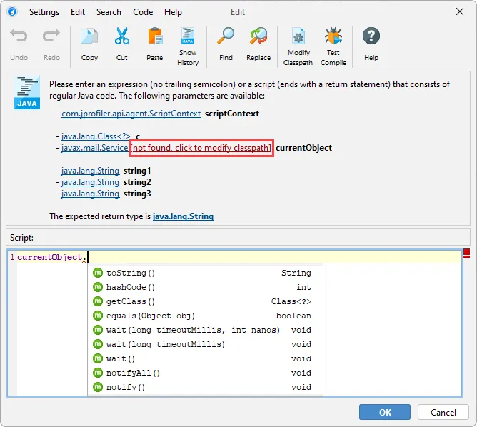
An action to modify the session classpath has been added to all script editors. Many features in JProfiler allow you to enter a
script for various purposes. For example, the "Split method with a script" action is available in the context menu of the call tree view.
If the class of the method or a class of a parameter is not in the configured session classpath, JProfiler cannot provide code completion
or compile a script that uses its members.
To solve this problem conveniently, JProfiler now adds action labels to modify the session classpath right next to the missing classes in the
script header. After adding the relevant JAR files to the classpath, you will be able to use the classes in the script immediately.
Attach mode was improved.
In the list of attachable JVMs, JProfiler now shows the JRE path when no other naming information about the application is available.
Because many applications use a private JRE, this makes it possible to identify those applications.
On Linux, you can now attach to processes that were started by systemd with "PrivateTmp=yes" in the systemd unit file. You have to use
the root user to attach to such processes.
Also on Linux, JProfiler now inspects the mounts that were namespaced per-process to find writable directories. This affects daemons launched
by systemd with "ProtectSystem=strict" in their system unit file, for example.
Added support for Linux Alpine ARM.
JVMs on this architecture can now be profiled by JProfiler.